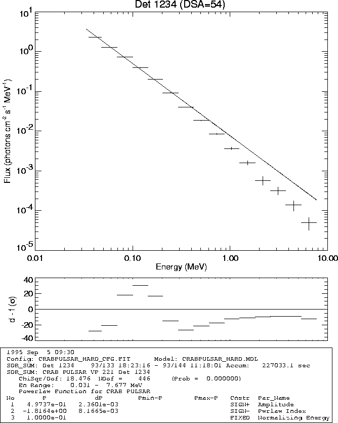
Figure 5.1: A Spectrum of the Crab Nebula & pulsar from Viewing Period 221. This was performed with the expanded response matrix.
If your target has significant emission up in the several MeV range (targets such as the Crab pulsar or the Sun), problems can arise due to the finite size of the detector response matrix. The default settings for SPECANAL generates a response matrix covering the nominal energy range of the OSSE detector: 0.05-10 MeV in count space. Photons with energies above the detector's nominal energy range can generate counts at lower energies so generally the response matrix is created covers energies from 0.02-12.0 MeV with 460 logarithmically-spaced channels.
For this exercise, we will take the daily good-summed (GSM) count spectra and regenerate the response matrix expanding the photon energy range. To respecify the generation of the response matrix, we need to use the MTRX_NPHOT and MTRX_PRANGE parameters in FFIT_PREP. In this example, we will expand the energy range in photon space to cover 0.02 to 20.0 MeV with 600 channels. We will also select new names for the output files to separate them from the normal SPECANAL run.
Igore> status=ffit_prep(file='ogre$dat:nom_cfg.fp',$
Igore>     sdbfile='od10:[gimgr.crab]CRABPULSAR_221_GSM.SDB',$
Igore>     outfile='crabpulsar_hard_tot.sdb',$
Igore>     fileroot='crabpulsar_hard',$
Igore>     filesetup='none',$
Igore>     mtrx_nphot=600,$
Igore>     mtrx_prange=[0.02,20.0])
Once the new total file is generated, it is ready to use.
Igore>; now combine the individual detectors
Igore> sdr_load,'CRABPULSAR_HARD_TOT.SDB',sdr
Igore> sdr$create,r_out,1
Igore> sdr_sum,sdr,r_out,/matrix

Igore>; and fit the resulting SDR
Igore> stat=fitit(fileroot='CRABPULSAR_HARD',$
Igore>         sdr=r_out,$
Igore>         modelfile='PWRlaw.MOD')
The result of this fit is shown in Figure 5.1. How much does this expanded response matrix alter the fit? We can examine the contents of the text output files CRABPULSAR_SOFT_PHOT.DAT and CRABPULSAR_HARD_PHOT.DAT. From these we notice that the flux in a given energy band is different with the expanded response matrix, though for this observation, it is differs only by a small amount. That will be true for many OSSE observations. The effect is only strong for bright, hard sources , such as solar flares.
Figure 5.1: A Spectrum of the Crab Nebula & pulsar from Viewing Period 221.
This was performed with the expanded response matrix.
OD10:[GIMGR.GI_GUIDE_DEV]CRABPULSAR_HARD_PHOT.DAT;1

;    [Mon Aug 14 14:38:27 1995]
;columns: 1 = E_low(MeV), 2 = Width(MeV), 3 = Flux(pho/MeV/cm2/s),   4 = Sigma
15     rows
4          columns
   3.532876e-02   1.239002e-02   2.304310e+00   7.621887e-03
   4.771877e-02   2.134042e-02   1.287403e+00   3.693308e-03
   6.905919e-02   3.071807e-02   7.201910e-01   1.284941e-03
   9.977726e-02   4.433932e-02   3.891529e-01   1.063650e-03
   1.441166e-01   5.824104e-02   1.992370e-01   6.661410e-04
   2.023576e-01   9.044579e-02   9.211867e-02   4.396134e-04
   2.928034e-01   1.284606e-01   4.004344e-02   4.065113e-04
   4.212640e-01   1.863276e-01   1.845548e-02   3.678837e-04
   6.075916e-01   2.640166e-01   8.496242e-03   2.870063e-04
   8.716082e-01   3.596396e-01   3.656742e-03   2.816125e-04
   1.248917e+00   5.628425e-01   1.592188e-03   1.803348e-04
   1.811760e+00   7.825322e-01   5.771935e-04   1.376720e-04
   2.594291e+00   1.125891e+00   3.194376e-04   7.037019e-05
   3.720183e+00   1.622687e+00   1.388980e-04   3.919802e-05
   5.342870e+00   2.302968e+00   4.960678e-05   1.742393e-05

OD10:[GIMGR.GI_GUIDE_DEV]CRABPULSAR_SOFT_PHOT.DAT;1

;    [Mon Aug 14 14:35:35 1995]
;columns: 1 = E_low(MeV), 2 = Width(MeV), 3 = Flux(pho/MeV/cm2/s),   4 = Sigma
15     rows
4          columns
   3.532876e-02   1.239002e-02   2.315879e+00   7.661720e-03
   4.771877e-02   2.134042e-02   1.287981e+00   3.695189e-03
   6.905919e-02   3.071807e-02   7.202391e-01   1.285031e-03
   9.977726e-02   4.433932e-02   3.891836e-01   1.063726e-03
   1.441166e-01   5.824104e-02   1.991939e-01   6.659965e-04
   2.023576e-01   9.044579e-02   9.205822e-02   4.393271e-04
   2.928034e-01   1.284606e-01   4.003363e-02   4.064146e-04
   4.212640e-01   1.863276e-01   1.842380e-02   3.671801e-04
   6.075916e-01   2.640166e-01   8.467456e-03   2.859893e-04
   8.716082e-01   3.596396e-01   3.632584e-03   2.794470e-04
   1.248917e+00   5.628425e-01   1.572489e-03   1.779186e-04
   1.811760e+00   7.825322e-01   5.666818e-04   1.351443e-04
   2.594291e+00   1.125891e+00   3.122509e-04   6.881129e-05
   3.720183e+00   1.622687e+00   1.357605e-04   3.831739e-05
   5.342870e+00   2.302968e+00   4.871346e-05   1.710554e-05