THE LIFETIME OF THE EXOSAT SPACECRAFT
1. Background
EXOSAT's design specification was based on a two-year operational
phase. This had a number of major influences on the system
design, particularly on the requirements for orbit stability,
end-of-life solar array power and attitude/manoeuvre fuel.
This article examines the actual situation after 21 months of
operation and considers those factors which will determine the
ultimate lifetime expectancy of the mission.
2. Orbit Considerations
The EXOSAT orbit had to satisfy the following criteria:
- maximum time spent outside the Van Allen radiation belts.
- line of apsides (apogee-perigee line) close to perpendicular
to the ecliptic plane, to maximise the area of sky over
which lunar occultations could be effected.
- a Northern apogee such that a single, Northern hemisphere
ground station (Villafranca, Spain) could be used for
telemetry reception, telecommanding and tracking.
These criteria led to a choice of orbit with the nominal
characteristics as shown in table 1.
The constraints on the time of day of launch for 26th May 1983
are shown in Fig. 1 and were:
- the Solar Aspect Angle (SAA) during the initial transfer
orbit had to lie between 30* and 120%
- there should be no eclipse during the transfer orbit.
- the final orbit lifetime had to be greater than 2 years.
- the maximum eclipse duration in the final orbit had to be
less than 60 minutes from considerations of battery design.
The EXOSAT launch took place 1 minute prior to window closure and
the orbit achieved had the characteristics as shown in Table 1
and a lifetime of approximately 3 years.
TABLE 1
|
| Orbital Elements | Nominal | Achieved
(26.5.83) |
|---|
|
| Height of Perigee | 350 km | 346.6 km |
| Height of Apogee | 196235 km | 191708.7 km |
| Eccentricity | 0.9355 | 0.93433 |
| Inclination | 72.50 | 72.470 |
| Argument of Perigee | 286.50 | 286.360 |
| Orbit Period | 93.6 hrs | 90.6 hrs |
|
EXOSAT's orbit is perturbed strongly by the gravitational
influence of the Sun and the Moon and this has the
(principal) effect of changing the eccentricity of the
orbit whilst the semimajor axis remains essentially
constant. Thus the perigee height has increased from 350
km initially to a maximum of ca. 4500 km in November 1984,
since when it has gradually decreased such that without
active control, the EXOSAT spacecraft will re-enter the
Earth's atmosphere during the second-half of April 1986
(see Fig. 2).
EXOSAT has, however, a hydrazine reaction control system
with a capability of imparting 173 m/sec to the orbit.
This system was included to permit active orbit control in
order to modify the orbit period by.small increments to
achieve the geometry required for moon occultation of Xray
sources. Hydrazine usage to date has been 2.3 m/sec
for commissioning and calibrating the system.
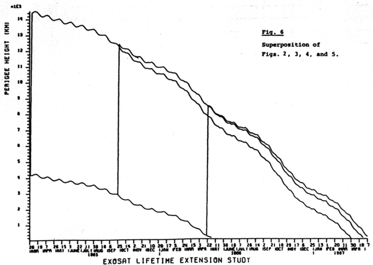
If the remaining 170 m/sec were used for perigee-raising,
the lifetime of the orbit could be extended by about 1
year ie. until April 1987. The amount of the extension
increases slightly the later the orbit manoeuvres are
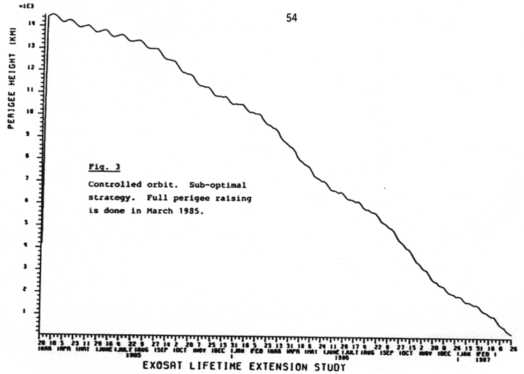
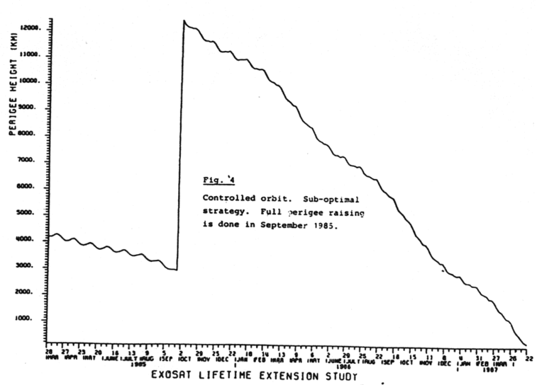
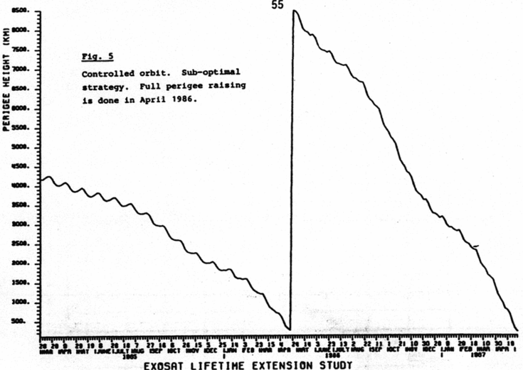
delayed; this effect is demonstrated in Figures 3 to 6.
The optimal strategy is to perform small manoeuvres
starting in April 1986 such that the perigee height is
maintained just above the critical value at which the
orbit would decay due to atmospheric friction (a few
hundred kilometres). Other considerations, however, will
probably dictate that less than the full 170 m/sec is used
to extend the lifetime (see Section 5 below).
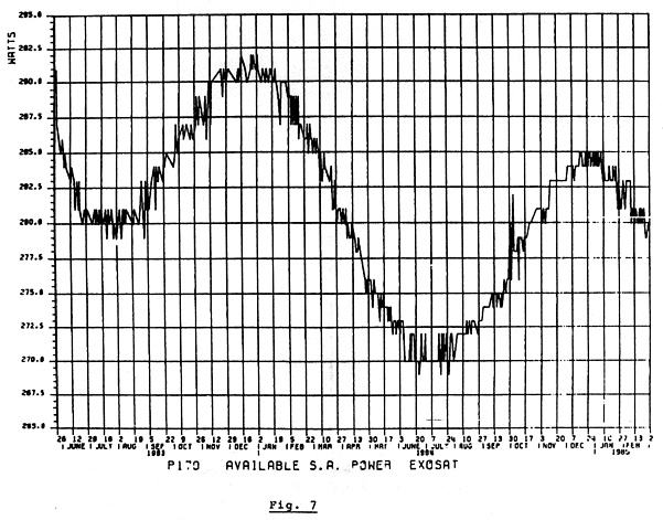
3. Power from the Solar Array
With the exception of eclipses (when battery power is
used) the subsystems and experiments are powered from
the Solar Array (consisting of 3312 solar cells) mounted
on top of the spacecraft and rotated such that it
remains near-normal to the Sun direction.
The output from the Array varies
because of:
- degradation of the solar cells from aging and
irradiation.
- variation in the Solar input caused by the
eccentricity of the Earth's orbit around the
Sun. This effect produces a variation of ca. 7%
in Solar input from perihelion (2nd January) to
aphelion.
The superposition of these two effects since launch can
be seen in Fig. 7, which shows the Array output as
derived from the Sun bus current and voltage sensors.
The "noise" on this curve is the combined
effect of telemetry quantisation, Array offsets from normal (up to
5°) and occasional high readings taken close to perigee
when there is a significant input to the Array from
Earth albedo.
The power currently required from the Array is around
230 Watts. This is not a constant load figure but
includes also the "peaks" which occur as a result of
aperiodic operation of thrusters and the temperature control circuits
of the gyros and therefore represents
the level at which battery discharge will not occur.
From the trend of the Array output to date, it can be
seen that this load can be supported throughout the
remaining natural mission lifetime and any possible
extension.
4. Attitude Control Fuel
Limit-cycling and attitude manoeuvres (slews) are
achieved using a cold-gas propane reaction control
system. 14 kilograms of propane were loaded, with a prelaunch
allocation between attitude manoeuvres and
attitude stabilisation of approximately 55%:45%. This
manoeuvre allocation was based on a (nominal) slew rate
of 300 deg/hr. In practice, the amount of fuel used for
manoeuvres has been somewhat less, since the slew rates
used have been lower (171 deg/hr was eliminated in Dec.
1984). However a number of anomalies which have occurred
with the Attitude and Orbit Control System, (AOCS, see
earlier reports) have used additional propane fuel, for
which there was no allowance in the original budget.
Although there is no direct measure of either the amount
of propane used or the amount remaining in the tanks,
two indirect but somewhat inaccurate methods are
available:
- Propane logging. Measurements have been made of
the fuel consumption for limit-cycling and
manoeuvring. This involves an operational
procedure whereby the commanded propane plenum
pressure is reduced for a short time and the rate
of fall of the pressure is monitored. A
housekeeping exercise is then carried out to
integrate the consumption over time, adding in
separately estimates for the additional fuel used
as a result of anomalies (spurious triggering of
Safety Mode, thrusters "stuck-on" etc). This
method indicates that approximately 5.5 kg of
propane remains as of-the middle of February
1985.
- Propane gauging.The propane tanks are
equipped with heaters with a total rating of 2.4
Watts, which are normally switched on only during
eclipses. Switching on these-heaters and
monitoring the subsequent temperature rise
(equilibrium is reached after about 4 days)
allows an estimate of the propane remaining in
the tanks.
Such an exercise was undertaken in the middle of
February 1985 and the preliminary results give a
"best fit" to a remaining propane mass of 4 kg.
These exercises are currently being re-examined in an
attempt to reconcile the substantially differing results.
Meanwhile, two measures are being applied to reduce the
rate of consumption:
- reduction of the manoeuvre frequency during the
forthcoming A03 programme, ie. increase the mean
observation duration, and limitation of the slew
rate to 42.7 deg/hr.
- Use of the Fine Sun Sensor for roll control (with
the OBC program SMC compensating for sun motion)
whenever possible. This measure results in lower
noise injection into the X-axis limit cycle than
the alternative 2-star roll control technique.
In this manner the overall consumption can be reduced to
just over 2 kg per year for future operations, assuming of
course that no further fuel-consuming anomalies occur.
Analysis of the calibration orbit manoeuvre indicates
that, if all of the 170 m/sec were utilised, this could
cost up to 1 k9 of propane for attitude stabilisation
during the orbit manoeuvre. This fuel is required to
compensate for the misalignment between the line of action
of the hydrazine thruster and the spacecraft centre of
mass.
5. Conclusions
The optimum use of the remaining propane will have been
made if the spacecraft re-enters the atmosphere at exactly
the same time as the propane is exhausted.
One method of achieving this would be to leave the orbit
uncontrolled until April 1986 and then to apply small
orbit corrections to extend the life until such time as
the propane is exhausted.
The approach however has two risk factors associated with it:
- with only a single actuation to date, there is
not yet a high confidence associated with the
operation of the hydrazine system. Failure of a
single manoeuvre late in the mission could be
irrecoverable.
- it is not possible to perform orbit manoeuvres
unless there are 3 operable gyros available to
control the attitude. The X-gyro spin motor
current rose dramatically on day 366 1984 and has
displayed an erratic behaviour since. In the
middle of February, it rose again and caused a
significant temperature increase of the gyro box
as a result of which the X-gyro was switched off.
Prior to this step however, there was good reason
to believe that the X-gyro could still be used to
control the spacecraft. If a second gyro fails,
it may be possible to "resurrect" the X-gyro to
reestablish 3-axis gyro control.
All factors considered, the current philosophy is to leave
the orbit uncontrolled until at least early 1986. If the
anomalous consumption of propane has then been minimal
throughout 1985, the strategy can be reviewed in the light
of the best estimate of the propane remaining at that
time.
A. Parkes
Fig.1 EXOSAT Launch Window