

THE XMM-NEWTON ABC GUIDE, STREAMLINED
Fit an EPIC Spectrum with Sherpa (Locally Installed)
For this example, we will first do a quick fit to see what we are dealing with, so we will rebin the data and use the default Gehrels χ2 statistics. Then, once we have an idea what the fit generally looks like and what should be reasonable inital values for the model parameters, we will redo the fit with cstat and considering the background spectrum.
First, it is convenient to edit the headers so Sherpa will automatically load the auxilliary files.
   > ciao
   > dmhedit mos1_pi.fits filelist=none operation=add key=BACKFILE value=bkg_pi.fits datatype=indef
   > dmhedit mos1_pi.fits filelist=none operation=add key=RESPFILE value=mos1_rmf.fits datatype=indef
   > dmhedit mos1_pi.fits filelist=none operation=add key=ANCRFILE value=mos1_arf.fits datatype=indef
Next, use Sherpa to bin and fit the spectrum, editting the parameters as needed.
> sherpa
> load_pha("mos1_pi.fits") ! input data
> calc_data_sum() ! find how many counts are in the spectrum
> group_counts(30) ! bin the data to a minimum of 30 counts per bin
> ignore(":0.2,3:") ! set a range appropriate for the data, in keV
> plot_data() ! plot the binned data
> set_source(xspowerlaw.p1) ! set spectral model to a power law
> p1.phoindex=2.0 ! set the initial value of the powerlaw photon index to 2.0
> p1.norm=1.e-5 ! set the initial value of the powerlaw normalization to 1.e-5
> fit() ! fit the model to the data
> covar() ! find the confidence intervals for all thawed parameters
> calc_energy_flux(lo=0.2,hi=3) ! find the energy flux (in erg/cm2/s) over the energy
! range 0.2-3 keV
> set_ylog() ! set the y axis to log scale for a different view
> set_xlog() ! set the x axis to log scale for a different view
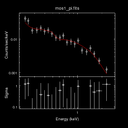
> plot_fit_delchi() ! plot two panels with the fit and the delta chi (residuals divided
! by uncertainties)
The fit and Δ χ are shown in Figure 1 (left).
Next, we will change the statistic and grouping, and consider the background.
> clean() ! erase the data and model settings
> load_pha("mos1_pi.fits")
> ignore(":0.2,3:")
> set_stat("cstat") ! change from "chi2gehrels" to "cstat"
> set_source(xspowerlaw.p1)
> set_bkg_model(xspowerlaw.p2) ! set the background model to a power law (using the same response
! files as the source)
> p1.phoindex=2.6
> p1.norm=3.e-5
> p2.phoindex=1.5
> p2.norm=1.e-6
> fit() ! both the source and background are fit automatically
> covar()
> calc_energy_flux(lo=0.2,hi=3)
> calc_energy_flux(lo=0.2,hi=3,bkg_id=1) ! find the background energy flux (in erg/cm2/s)
! over the energy range 0.2-3 keV
> set_ylog()
> set_xlog()
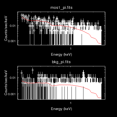
> plot("fit",1,"bkgfit",1) ! plot the fits to the source and background in the same window
> exit
The fit is shown in Figure 1 (right).
|
If you have any questions concerning XMM-Newton send e-mail to xmmhelp@lists.nasa.gov