THE XMM-NEWTON ABC GUIDE, STREAMLINED
EPIC-MOS (TIMING mode), Hera Parameter Window

Prepare the Data
Reprocess the Data
Make a Light Curve
Apply Standard Filters
Apply Time Filters
Extract the Source and Background Spectra
Determine the Spectrum Extraction Areas
Check for Pile Up
Create the Photon Redistribution Matrix (RMF) and Ancillary File (ARF)

Prepare the Data

Please note that the two tasks in this section (cifbuild and odfingest) must be run in the ODF directory. These are the only tasks with that requirement, and after this section, we will work exclusively in our reprocessing directory.

Many SAS tasks require calibration information from the Calibration Access Layer (CAL). Relevant files are accessed from the set of Current Calibration File (CCF) data using a CCF Index File (CIF). To make the ccf.cif file, navigate into the ODF directory using the icons in the User Account Window of the Hera interface. Then, in the Tool Parameter Window, in the Task Name box, enter cifbuild and click "Get".

The task odfingest extends the Observation Data File (ODF) summary file with data extracted from the instrument housekeeping data files and the calibration database. It is only necessary to run it once on any dataset, and will cause problems if it is run a second time. If for some reason odfingest must be rerun, you must first delete the earlier file it produced. This file largely follows the standard XMM naming convention, but has SUM.SAS appended to it. To run odfingest, in the Tool Parameter Window, in the Task Name box, enter odfingest and click "Change".

Hera automatically resets the relevant environmental parameters to the output of these tasks, so we can continue merrily on our way.

Reprocess the Data

To reprocess the data, go up one directory in the tree and make a new working directory using the buttons in the upper left corner of the User Account Window. When you are in the working directory, call either emproc or emchain As in the previous section, just enter the task name in Task Name box and click "Change".

By default, these tasks not keep any intermediate files they generate. Emchain maintains the usual naming convention. Emproc designates its output event files with "TimingEvts.ds". In any case, it is convenient to rename them something easy to type; this can be done by clicking on the pen icon next to the file name in the User Account Window. We'll assume the new name for the event file is mos1_te.fits.

If you are likely to want to extract a background spectrum for your source, you will also need to consider the imaging event file. We might as well deal with that while we're here. Remember that whatever filtering is done on the timing event file must also be done on the image event file. We will rename the image event file mos1_ie.fits.

Make a Light Curve

The XMM-Newton Observatory is susceptible to soft particle flaring, so it is necessary to examine the light curve to determine how much of the data is useful.

To create a light curve, enter evselect into the Task Name box and click "Change". Then,

By the table parameter, use the Browse button to select the event file, mos1_te.fits.
Set withrateset to yes. This will make the parameters that are relevant specifically to making a light curve appear.
Set maketimecolumn to yes, set timebinsize to 20, and enter an output file name in rateset. We will use mos1_ltcrv.fits.
Click "Run evselect".

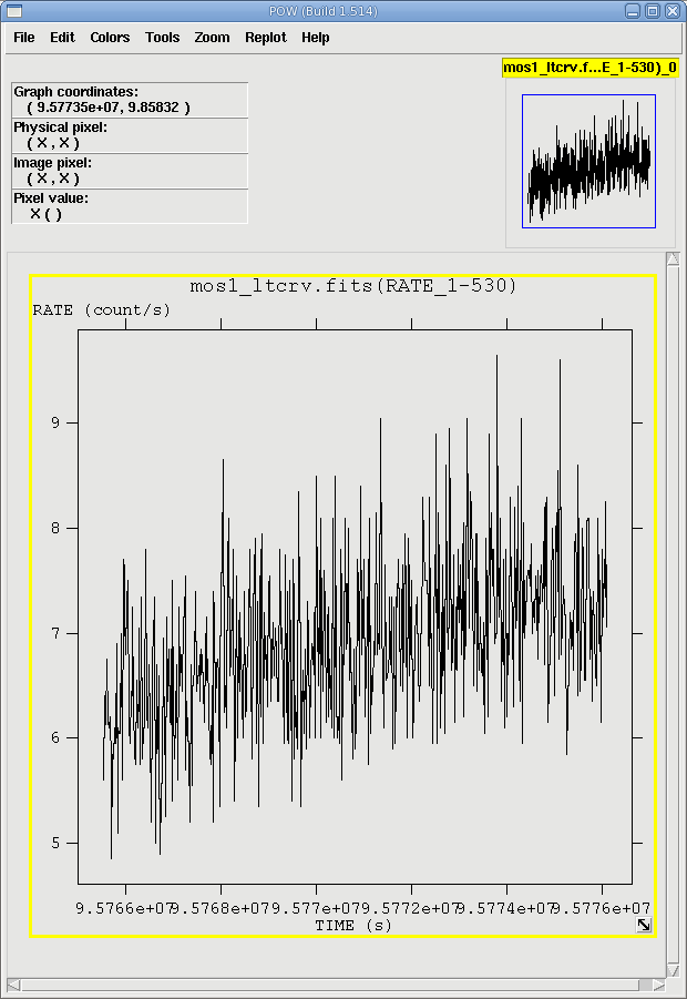
The output file mos1_ltcrv.fits can be viewed by downloading and displaying it with fv on your local machine.

   fv mos1_ltcrv.fits &

In the pop-up window, the RATE extension will be available in the second row (index 1, as numbering begins with 0). Selecting PLOT from this row will let you choose the column name and axis on which to plot it. The light curve is shown in Figure 1.

**Figure 1:** The Mkn 841 light curve.

Apply Standard Filters

The filtering expression for the MOS in TIMING mode is:

(PATTERN <= 12)&&(PI in [200:12000])&&#XMMEA_EM

The first two expressions will select good events with PATTERN in the 0 to 12 range. The PATTERN value is similar the GRADE selection for ASCA data, and is related to the number and pattern of the CCD pixels triggered for a given event. Single pixel events have PATTERN == 0, while double pixel events have PATTERN in [1:4] and triple and quadruple events have PATTERN in [5:12].

The second keyword in the expressions, PI, selects the preferred pulse height of the event. For the MOS, it should be between 200 and 12000 eV. This should clean up the image significantly with most of the rest of the obvious contamination due to low pulse height events. Setting the lower PI channel limit somewhat higher (e.g., to 300 or 400 eV) will eliminate much of the rest.

Finally, the #XMMEA_EM filter provides a canned screening set of FLAG values for the event. (The FLAG value provides a bit encoding of various event conditions, e.g., near hot pixels or outside of the field of view. Setting FLAG == 0 in the selection expression provides the most conservative screening criteria and usually is not necessary for the MOS.)

To filter the data, enter evselect into the Task Name box and click "Change". Then,

By the table parameter, use the Browse button to select the event file, mos1_te.fits.
Set keepfilteroutput to yes. This will make the parameters that are relevant specifically to filtering a file appear.
Set withfilteredset to yes. Enter an output file name in filteredset, mos1_te_filt.fits. In the expression parameter box, enter (PATTERN <= 12) && (PI in [200:12000]) && #XMMEA_EM
Click "Run evselect".

Remember to run the same filter on the image event file if you plan to use it. We will refer to the filtered image event file as mos1_ie_filt.fits.

Apply Time Filters

Sometimes, soft proton background flaring makes it necessary to use filters on time in addition to those mentioned above.

To determine if there is flaring in the observation, make a light curve and display it. No flares are evident, so we will continue to the next section. However, if a given dataset does contain flaring, it should be removed in the same way as shown for EPIC IMAGING mode data.

Extract the Source and Background Spectra

First, we will need to make an image of the filtered event file. Enter evselect into the Task Name box and click "Change". Then,

By the table parameter, use the Browse button to select the event file, mos1_te_filt.fits.
Set withimageset to yes. This will make parameters that are specific to making an image appear.
Enter an output file name in imageset. We will use mos1_te_image.fits. Confirm that xcolumn is set to RAWX and ycolumn is set to TIME, and ximagebinsize and yimagebinsize are set to 1.
Click "Run evselect".

**Figure 2:** Mkn 841 timing data.

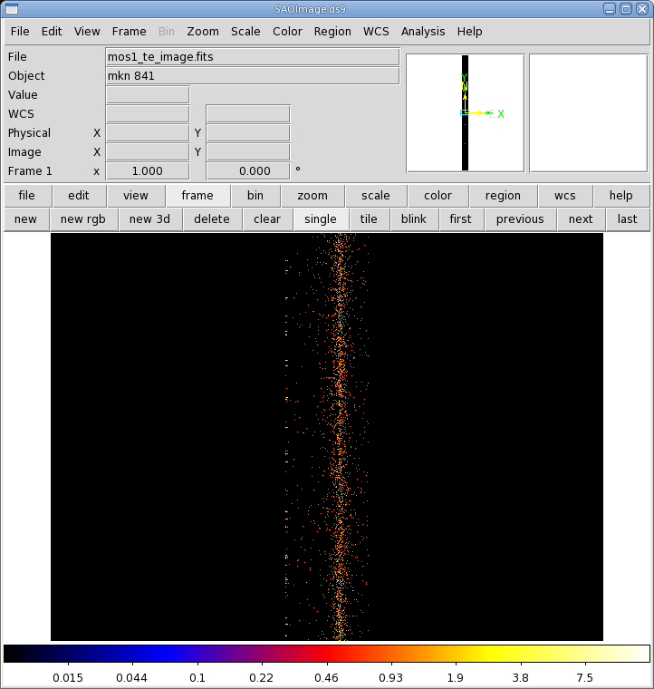
The image can be downloaded and displayed with ds9. As can be seen in Figure 2, the source is centered on RAWX=314. We will extract this and the 2 pixels on either side of it.

By the table parameter, use the Browse button to select the event file, mos1_te_filt.fits.
Set keepfilteroutput, withfilteredset, and withspectrumset to yes. This will make parameters that are specific to filtering an event file and extracting a spectrum appear. Set withspecranges to yes.
Enter an event file output name in filteredset. We will use mos1_te_filt_source.fits. Enter a spectrum output file name in spectrumset. We will use source_pi.fits. Set energycolumn to PI. In the expression parameter box, enter (FLAG==0) && (RAWX in [304:324]). Set specchannelmax to 11999.
Click "Run evselect".

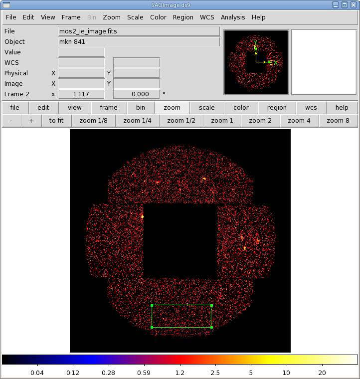
If needed, we can also extract a background spectrum. For this, we will use the imaging event list, since we want the background to be as far away from the source as possible. As with the source spectrum, we will need to make an image first.

By the table parameter, use the Browse button to select the event file, mos1_ie_filt.fits.
Set withimageset to yes. This will make parameters that are specific to making an image appear.
Enter an output file name in imageset. We will use mos1_ie_image.fits. Confirm that xcolumn is set to RAWX and ycolumn is set to TIME, and ximagebinsize and yimagebinsize are set to 1.
Click "Run evselect".

The image is shown in Figure 3, with the background extraction region overlayed. Now for the spectrum:

By the table parameter, use the Browse button to select the event file, mos1_ie_filt.fits.
Set keepfilteroutput, withfilteredset, and withspectrumset to yes. This will make parameters that are specific to filtering an event file and extracting a spectrum appear. Set withspecranges to yes.
Enter an event file output name in filteredset. We will use mos1_ie_filt_source.fits. Enter a spectrum output file name in spectrumset. We will use bkg_pi.fits. Set energycolumn to PI. In the expression parameter box, enter (FLAG==0) && ((DETX,DETY) in BOX(301.5,-13735.5,10700,4000,0)). Set specchannelmax to 11999.
Click "Run evselect".

**Figure 3:** The filtered imaging event file for Mkn 841. The green box indicates the region where the background spectrum was extracted.

Determine the Spectrum Extraction Areas

The source and background region areas can now be found. (This process is identical to that used for IMAGING data.) This is done with the task backscale, which takes into account any bad pixels or chip gaps, and writes the result into the BACKSCAL keyword of the spectrum table. To find the source and background extraction areas, enter backscale in the Task Name box and click "Change". Then,

Check for Pile Up

Depending on how bright the source is and what modes the EPIC detectors are in, event pile up may be a problem. Pile up occurs when a source is so bright that incoming X-rays strike two neighboring pixels or the same pixel in the CCD more than once in a read-out cycle. In such cases the energies of the two events are in effect added together to form one event. Pile up and how to deal with it are discussed at length here and here, respectively, and users are strongly encouraged to refer to those sections. Briefly, we deal with it in MOS TIMING data essentially the same way as in IMAGING data, that is, by using only single pixel events, and/or removing the regions with very high count rates, checking the amount of pile up, and repeating until it is no longer a problem.

In our example case, the source is far too faint to be piled up, but it is always a good idea to check anyway.

To check for pile up, enter epatplot in the Task Name box and click "Change". Then,

Create the Photon Redistribution Matrix (RMF) and Ancillary File (ARF)

Making the RMF for MOS data in TIMING mode is exactly the same as in IMAGING mode, which is demonstrated here. If the boresight was not excised (as may be necessary if your data is piled up), making the ARF is the same, as well.

Now use the RMF, spectrum, and event file to make the ancillary file. Enter arfgen in the Task Name box and click "Change". Then,

However, if you had to remove piled up sections, you will need to make an ARF for the full extraction area, another one for the piled up area, and then subtract the two to find the ARF for the non-piled regions. Users are referred to this discussion, where the procedure is demonstrated on PN TIMING data.

The spectrum can be fit using HEASoft or CIAO packages, as SAS does not include fitting software.

THE XMM-NEWTON ABC GUIDE, STREAMLINED EPIC-MOS (TIMING mode), Hera Parameter Window

Contents