

THE XMM-NEWTON ABC GUIDE, STREAMLINED
OM (FAST Mode), Command Window
Contents
Prepare the Data
OM Artifacts and General Information
Reprocess the Data
Verify the Output
Prepare the Data
Please note that the two tasks in this section (cifbuild and odfingest) must be run in the ODF directory. These are the only tasks with that requirement, and after this section, we will work exclusively in our reprocessing directory.Many SAS tasks require calibration information from the Calibration Access Layer (CAL). Relevant files are accessed from the set of Current Calibration File (CCF) data using a CCF Index File (CIF). Setting the environment paraters follows the same syntax as the cshell in linux. To set the environment parameters and make the ccf.cif file, navigate into the ODF directory and in the Command Window, type
   setenv SAS_ODF /data/0411081601/ODF
   setenv SAS_ODFPATH /data/0411081601/ODF
   cifbuild
To use the updated CIF file in further processing, you will need to reset the environment variable SAS_CCF:
setenv SAS_CCF /data/0411081601/ODF/ccf.cifThe task odfingest extends the Observation Data File (ODF) summary file with data extracted from the instrument housekeeping data files and the calibration database. It is only necessary to run it once on any dataset, and will cause problems if it is run a second time. If for some reason odfingest must be rerun, you must first delete the earlier file it produced. This file largely follows the standard XMM naming convention, but has SUM.SAS appended to it. To run odfingest and reset the environment variable:
   odfingest
   setenv SAS_ODF /data/0411081601/ODF/1358_0411081601_SCX00000SUM.SAS
OM Artifacts and General Information
Before proceeding with the pipeline, it is appropriate to discuss the artifacts that often affect OM images. These can affect the accuracy of a measurement by, for example, increasing the background level.
- Stray light. Background celestial light is reflected by
the OM detector housing onto the center on the OM field of view, producing a circular
area of high background. This can also produce looping structures and long streaks.
- Modulo 8 noise. In the raw images, a modulo 8 pattern
arises from imperfections in the event centroiding algorithm in the OM electronics.
This is removed during image processing.
- Smoke rings. Light from bright sources is reflected from the entrance
window back on the detector, producing faint rings located radially away from the center
of the field of view.
- Out-of-time events. sources with count rates of several tens
of counts/sec show a strip of events along the readout direction, corresponding to
photons that arrived while the detector was being read out.
Users should also keep in mind some differences between OM data and X-ray data. Unlike EPIC and RGS, there are no good time intervals (GTIs) in OM data; an entire exposure is either kept or rejected. Also, OM exposures only provide direct energy information when in grism mode, and the flat field response of the detector is assumed to be unity.
Reprocess the Data
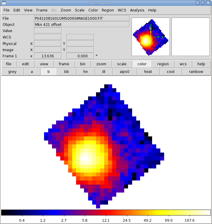
The repipelining task for OM data taken in fast mode is omfchain. It produces images of the detected sources, extracts events related to the sources and the background, and extracts the corresponding light curves. At present, unlike omichain, omfchain does not allow for keywords to specify filters or exposures; calling this task will process all fast mode data.Use the interface buttons in the User Account Window to make a new working directory, and double-click on it to open it. Then, in the Command Window, type
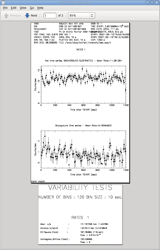
omfchainThere are two types of output files: those that start with F are intermediate images or time series files; those that start with P are products. The processed image in sky-coordinates from one exposure, P0411081601OMS006SIMAGE1000.FIT, and the background-subtracted light curve and various statistics associate with it, F0411081601OMS006TIMESR1000.PS, are shown in Figure 1.
|
Verifying the Output
A good first step is to examine the light curve plot for both the source and background, making sure they are reasonable: no isolated, unusually high (or low) values, and no frequent drop-outs. Users should also check the image in the Fast mode window to see if the source is near an edge. If it is, it's a good idea to examine the light curves from diffent exposures to verify that they are consistent from exposure to exposure (while keeping in mind any intrinsic source variability). If the image is blurred or unusual in any way, users should check the tracking history file to verify the tracking was reliable.If you have any questions concerning XMM-Newton send e-mail to xmmhelp@lists.nasa.gov