

THE XMM-NEWTON ABC GUIDE, STREAMLINED
OM (IMAGING Mode), Hera Parameter Window
Contents
Prepare the Data
OM Artifacts and General Information
Reprocess the Data
Verify the Output
Prepare the Data
Please note that the two tasks in this section (cifbuild and odfingest) must be run in the ODF directory. These are the only tasks with that requirement, and after this section, we will work exclusively in our reprocessing directory.Many SAS tasks require calibration information from the Calibration Access Layer (CAL). Relevant files are accessed from the set of Current Calibration File (CCF) data using a CCF Index File (CIF). To make the ccf.cif file, navigate into the ODF directory using the icons in the User Account Window of the Hera interface. Then, in the Tool Parameter Window, in the Task Name box, enter cifbuild and click "Get".
The task odfingest extends the Observation Data File (ODF) summary file with data extracted from the instrument housekeeping data files and the calibration database. It is only necessary to run it once on any dataset, and will cause problems if it is run a second time. If for some reason odfingest must be rerun, you must first delete the earlier file it produced. This file largely follows the standard XMM naming convention, but has SUM.SAS appended to it. To run odfingest, in the Tool Parameter Window, in the Task Name box, enter odfingest and click "Change".
Hera automatically resets the relevant environmental parameters to the output of these tasks, so we can continue merrily on our way.
OM Artifacts and General Information
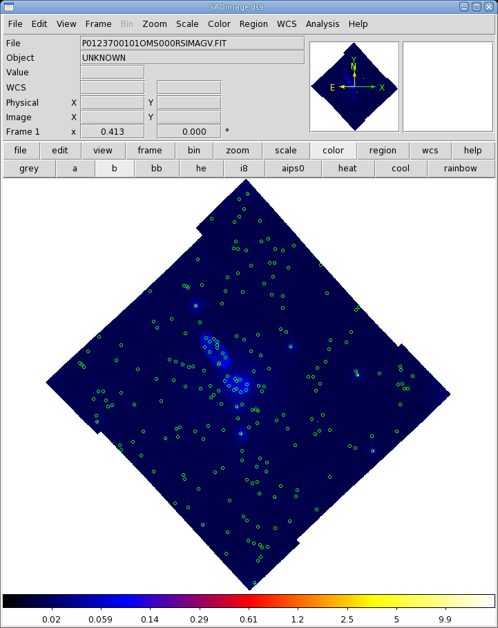
Before proceeding with the pipeline, it is appropriate to discuss the artifacts that often affect OM images. These can affect the accuracy of a measurement by, for example, increasing the background level. Some of these can be seen in Figure 1.
- Stray light. Background celestial light is reflected by
the OM detector housing onto the center on the OM field of view, producing a circular
area of high background. This can also produce looping structures and long streaks.
- Modulo 8 noise. In the raw images, a modulo 8 pattern
arises from imperfections in the event centroiding algorithm in the OM electronics.
This is removed during image processing.
- Smoke rings. Light from bright sources is reflected from the entrance
window back on the detector, producing faint rings located radially away from the center
of the field of view.
- Out-of-time events. sources with count rates of several tens
of counts/sec show a strip of events along the readout direction, corresponding to
photons that arrived while the detector was being read out.
Users should also keep in mind some differences between OM data and X-ray data. Unlike EPIC and RGS, there are no good time intervals (GTIs) in OM data; an entire exposure is either kept or rejected. Also, OM exposures only provide direct energy information when in grism mode, and the flat field response of the detector is assumed to be unity.
If you simply want a quick look at your data, sky images and source lists are in *SIMAGE*.FTZ and *SWSRLI*.FTZ, respectively. Further, there are low resolution sky images for each filter; they follow the nomenclature:
PjjjjjjkkkkOMX000RSIMAGbb000.QQQ
where
-
jjjjjj - Proposal number
kkkk - Observation ID
b - Filter keyword: B, V, U, M (UVM2), L (UVW1) and S (UVW2)
QQQ - File type (e.g., PNG, FTZ)
To see what files have been summed to make the final image, search for the keyword XPROC0 in the FITS header. In Hera, the FITS header can be seen by clicking on the "i" icon.
For our example image, this would be
   XPROC0  = 'ommosaic imagesets=''/.hera_mountpnt/hera_users/testhera/data/01237&'
   CONTINUE  '00101/reproc_webhera_PW_OM/P0123700101OMS004SIMAGE1000.FIT /.hera_m&'
   CONTINUE  'ountpnt/hera_users/testhera/data/0123700101/reproc_webhera_PW_OM/P0&'
   CONTINUE  '123700101OMS415SIMAGE1000.FIT /.hera_mountpnt/hera_users/testhera/d&'
   CONTINUE  'ata/0123700101/reproc_webhera_PW_OM/P0123700101OMS416SIMAGE1000.FIT&'
   CONTINUE  ' /.hera_mountpnt/hera_users/testhera/data/0123700101/reproc_webhera&'
   CONTINUE  '_PW_OM/P0123700101OMS417SIMAGE1000.FIT /.hera_mountpnt/hera_users/t&'
   CONTINUE  'esthera/data/0123700101/reproc_webhera_PW_OM/P0123700101OMS418SIMAG&'
   CONTINUE  'E1000.FIT'' mosaicedset=/.hera_mountpnt/hera_users/testhera/data/01&'
   CONTINUE  '23700101/reproc_webhera_PW_OM/P0123700101OMS000RSIMAGV.FIT correlse&'
   CONTINUE  't='''' nsigma=2 mincorr=0 minfraction=0.5 maxdx=5 binaxis=0 numinte&'
   CONTINUE  'rvals=2 di=10 minnumpixels=100 # (ommosaic-2.5.18) [xmmsas_20131209&'
   CONTINUE  '_1901-13.5.0]'
The source list file (*SWSRLI*.FTZ) also contains useful information. Some column names are listed in Table 1.
| Column name | Contents |
| SRCNUM | Source number |
| RA | RA of the detected source |
| DEC | Dec of the detected source |
| POSERR | Positional uncertainty |
| RATE | extracted count rate |
| RATE_ERR | error estimate on the count rate |
| SIGNIFICANCE | Significance of the detection (in σ) |
| MAG | Brightness of the source in magnitude |
| MAGERR | uncertainty on the magnitude |
Reprocess the Data
To reprocess the data, go up one directory in the tree and make a new working directory using the buttons in the upper left corner of the User Account Window. When you are in the working directory, call omichain. As in the previous section, just enter the task name in Task Name box and click "Change". The default parameters are fine for most datasets, so click "Run omichain".This produces numerous files, including images and regions for each exposure and each filter. Luckily, omichain will let you specify exposures, filters, and other parameters, so if you are interested only in, say, the sources detected in the mosaicked V band image, we could run omichain with the appropriate flags. In omichain's parameter window,
- Set filters to V. Confirm that processmosaicedimages is set to yes, omdetectnsigma is set to 2.0, and omdetectminsignificance is set to 3.0.
- Click "Run omichain".
The output files can be used immediately for analysis, though users are strongly urged to examine the output for consistancy first (see the next section). The chains apply all necessary corrections, so no further processing or filtering needs to be done. Please note that the chains do not produce output files with exactly the same names as those in the PPS directory. (They also produce some files which are not included in the PPS directory at all.) Table 2 lists the file ID equivalences between repipelined and PPS files.
| Repipelined | PPS Name | Description |
| Name | ||
| EVLIST | none | Fast mode events list |
| FIMAG_ | FIMAG_ | combined full-frame image |
| FLAFLD | none | flatfield |
| FSIMAG | FSIMAG | combined full-frame sky image |
| HSIMAG | HSIMAG | full-frame HIRES sky image mosaic |
| IMAGE_ | IMAGE_ | image from any filter or Grism |
| IMAGE_ | IMAGEF | Fast mode image |
| LSIMAG | LSIMAG | full-frame LORES sky image mosaic |
| OBSMLI | OBSMLI | combined observation source list |
| REGION | SWSREG | sources region file |
| REGION | SFSREG | Fast mode sources region file |
| REGION | SGSREG | Grism ds9 regions |
| RIMAGE | GIMAGE | Grism rotated image |
| RSIMAG | RSIMAG | default mode sky mosaic |
| SIMAGE | SIMAGE | sky aligned image |
| SIMAGE | SIMAGF | Fast mode sky aligned image |
| SIMAGE | none | Grism sky aligned image |
| SPCREG | SPCREG | Grism ds9 spectrum regions |
| SPECLI | SPECLI | Grism specra list |
| SPECTR | SPECTR | source extracted spectra |
| SUMMAR | SUMMAR | observation summary |
| SWSRLI | SWSRLI | sources list |
| SWSRLI | SFSRLI | Fast mode sources list |
| SWSRLI | SGSRLI | Grism sources list |
| TIMESR | TIMESR | Fast mode source timeseries |
| TSHPLT | TSHPLT | tracking history plot |
| TSTRTS | TSTRTS | tracking star timeseries |
Verifying the Output
While the output from the chains is ready for analysis, OM does have some peculiarities, as discussed above. While these usually have only an aesthetic effect, they can also affect source brightness measurements, since they increase the background. In light of this, users are strongly encouraged to verify the consistency of the data prior to analysis. There are a few ways to do this. Users can download and examine the combined source list with fv, which will let them see if interesting sources have been detected in all the filters where they are visible. Users can also overlay the image source list on to the sky image with ds9 by using slconv to change source lists into region files. The task slconv allows users to set the regions radii in arcseconds to a constant value or scale them to header keywords, such as RATE. By default, ds9 region files have suffixes of .reg. In the example below, we make a region file from the source list for the mosaicked, V-band sky image.To make a ds9 region file from a source list, enter slconv into the Task Name box, and click "Change". Then,
- Set srclisttab to P0123700101OMS000RSISWSV.FIT and radiusexpression to 5.
- Set outfileprefix to the prefix of the output file name; we will use Vband_mosaic. Confirm that outputstyle is set to ds9.
- Click "Run slconv".
|
If you have any questions concerning XMM-Newton send e-mail to xmmhelp@lists.nasa.gov