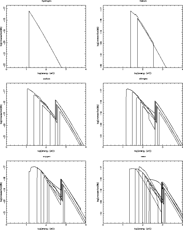
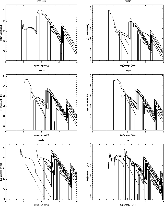
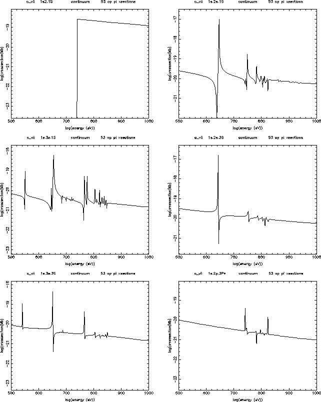
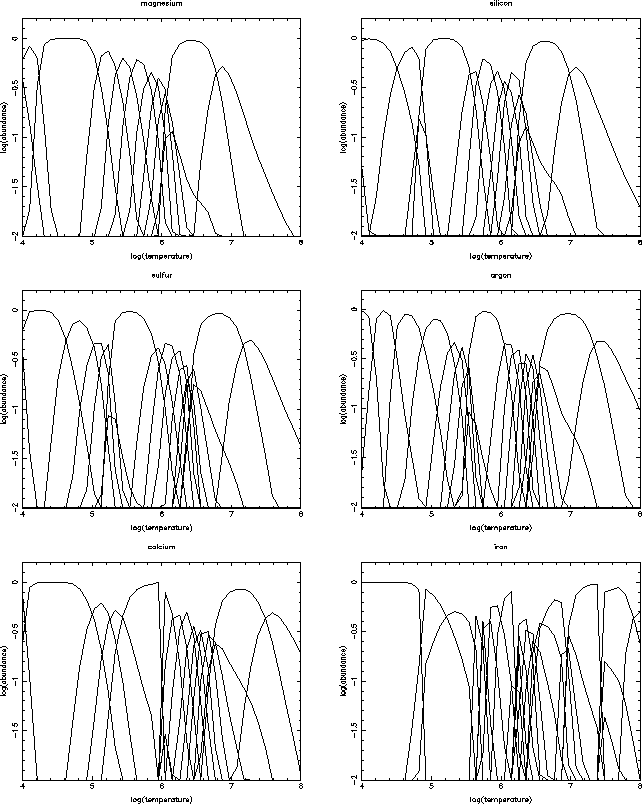
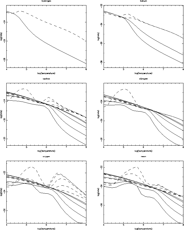
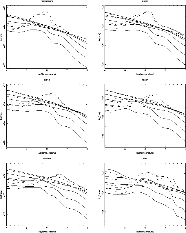
The effects of stimulated recombination

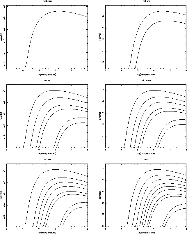
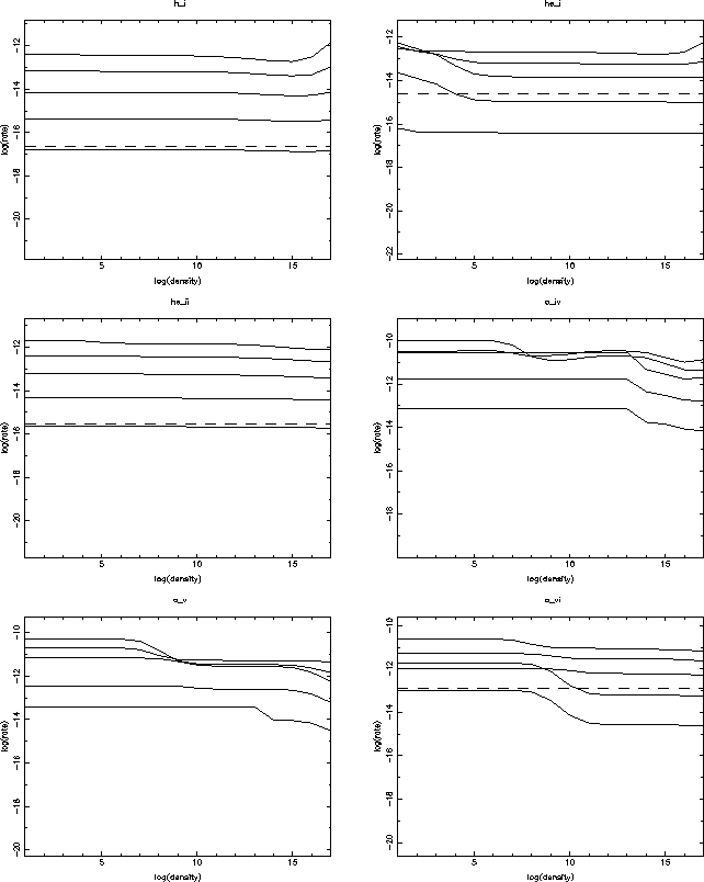
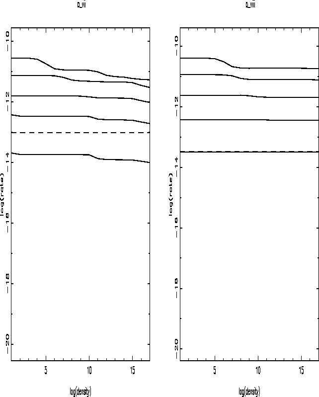
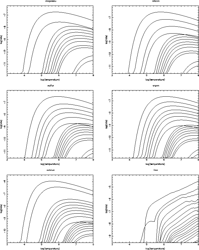
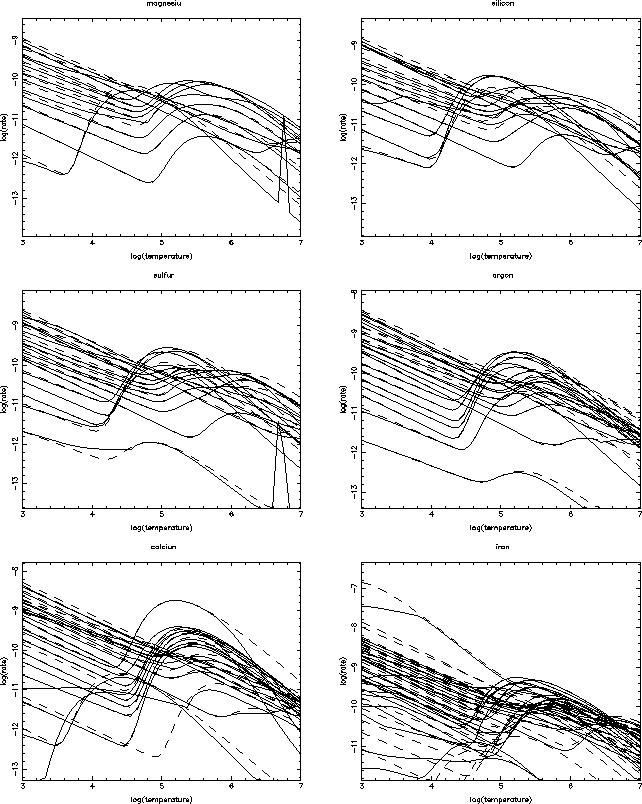
So far in this section we have artificially excluded the effects of stimulated recombination (by manually setting the rates to zero when calculating total recombination). We illustrate the effect of relaxing this condition in figure 16, which is the equivalent of figure 9 (recombination rates vs. density) but with stimulated recombination included. Again the ionizing spectrum is a $\varepsilon^{-1}$ power law, which has strong flux at the lowest photon energies. Comparison of figures 16 and 9 shows that the rates are greatly enhanced at high densities, and this enhancement is greatest for ions with lowest ionization potentials. This is due to the influence of the low energy photons on the stimulated recombination rate, and a different spectral shape (e.g. a blackbody) would produce a different distribution of recombination with charge state at high densities.

**Figure 1:** figure 1a
$\begin{figure} \epsfxsize =5.6in % narrow the plot\epsfysize =7.0in % shorten the plot \epsffile{fig1a.eps}\end{figure}$

**Figure 1:** figure 1b
$\begin{figure} \epsfxsize =5.6in % narrow the plot\epsfysize =7.0in % shorten the plot \epsffile{fig1b.eps}\end{figure}$

**Figure 2:** figure 2
$\begin{figure} \epsfxsize =5.6in % narrow the plot\epsfysize =7.0in % shorten the plot \epsffile{fig2.eps}\end{figure}$

**Figure 3:** figure 3a
$\begin{figure} \epsfxsize =5.6in % narrow the plot\epsfysize =7.0in % shorten the plot \epsffile{fig3a.eps}\end{figure}$

**Figure 3:** figure 3b
$\begin{figure} \epsfxsize =5.6in % narrow the plot\epsfysize =7.0in % shorten the plot \epsffile{fig3b.eps}\end{figure}$

**Figure 4:** figure 4a
$\begin{figure} \epsfxsize =5.6in % narrow the plot\epsfysize =7.0in % shorten the plot \epsffile{fig4a.eps}\end{figure}$

**Figure 4:** figure 4b
$\begin{figure} \epsfxsize =5.6in % narrow the plot\epsfysize =7.0in % shorten the plot \epsffile{fig4b.eps}\end{figure}$

**Figure 5:** figure 5a
$\begin{figure} \epsfxsize =5.6in % narrow the plot\epsfysize =7.0in % shorten the plot \epsffile{fig5a.eps}\end{figure}$

**Figure 5:** figure 5b
$\begin{figure} \epsfxsize =5.6in % narrow the plot\epsfysize =7.0in % shorten the plot \epsffile{fig5b.eps}\end{figure}$

**Figure 6:** figure 6a
$\begin{figure} \epsfxsize =5.6in % narrow the plot\epsfysize =7.0in % shorten the plot \epsffile{fig6a.eps}\end{figure}$

**Figure 6:** figure 6b
$\begin{figure} \epsfxsize =5.6in % narrow the plot\epsfysize =7.0in % shorten the plot \epsffile{fig6b.eps}\end{figure}$

**Figure 7:** figure 7a
$\begin{figure} \epsfxsize =5.6in % narrow the plot\epsfysize =7.0in % shorten the plot \epsffile{fig7a.eps}\end{figure}$

**Figure 7:** figure 7b
$\begin{figure} \epsfxsize =5.6in % narrow the plot\epsfysize =7.0in % shorten the plot \epsffile{fig7b.eps}\end{figure}$

**Figure 8:** figure 8a
$\begin{figure} \epsfxsize =5.6in % narrow the plot\epsfysize =7.0in % shorten the plot \epsffile{fig8a.eps}\end{figure}$

**Figure 8:** figure 8b
$\begin{figure} \epsfxsize =5.6in % narrow the plot\epsfysize =7.0in % shorten the plot \epsffile{fig8b.eps}\end{figure}$

**Figure 9:** figure 9a
$\begin{figure} \epsfxsize =5.6in % narrow the plot\epsfysize =7.0in % shorten the plot \epsffile{fig9a.eps}\end{figure}$

**Figure 9:** figure 9b
$\begin{figure} \epsfxsize =5.6in % narrow the plot\epsfysize =7.0in % shorten the plot \epsffile{fig9b.eps}\end{figure}$