Investigation of modeling the PCA background as a function of
recent SAA history.
Here is a summary of an attempt to model the PCA residual background
as a function of particle rate plus SAA related activation as
parameterized by the HEXTE particle monitor. The functional
form explored is
RATE = A + B * VLE_rate + SUM(i=1,3) ( Ci * SUMj(SAAj * exp ( (t-tj)/taui)
iThe index j runs over recent SAA doses which are either integrated on an orbit by orbit basis
or on a day by day basis. The calculation is not carried beyond 10 e-folding times.
For this investigation I take data from one of the repeated blank sky pointings
(20801-05-xx-xx). Data is selected subject to the constraint that the PCA is
viewing the sky ("ELV .gt. 10.0") and that more than about 30 minutes has
elapsed since the peak of the most recent pass through the SAA
("(BKGD_THETA .lt. -70.0 .or. BKGD_THETA .gt. 150.0) .or. time_since_saa .gt. 30.").
The second cut reduces the data set to 463 bins (from 544) of 256 seconds each.
Data is selected separately for each layer of PCU 0, 1, 2.
A summary of the results for these fits is given in the table. These fits include 463 independent points; all rates are expressed in units of counts/256 seconds.
          chi-sq     A                   B                     C_1                  tau_1                  C_2                   tau_2                 C_3                   tau_3

Pcu0 L1   1.805  2.04E+03+/- 4.90E+01  3.31E-02+/- 4.84E-04  1.53E-03+/- 2.29E-04  2.29E+01+/- 3.58E+00  3.61E-04+/- 3.65E-05  2.17E+02+/- 1.76E+01  1.22E-05+/- 2.69E-06  5.99E+03+/- 1.71E+03
Pcu0 L2   1.864  1.01E+03+/- 1.64E+01  2.16E-02+/- 3.15E-04  9.61E-04+/- 9.82E-05  2.44E+01+/- 2.08E+00  2.02E-04+/- 1.26E-05  2.44E+02+/- 1.39E+01  7.08E-06+/- 6.47E-07  7.26E+03+/- 6.63E+02
Pcu0 L3   1.651  9.31E+02+/- 3.03E+01  2.22E-02+/- 3.55E-04  6.55E-04+/- 8.22E-05  3.00E+01+/- 4.75E+00  1.88E-04+/- 2.17E-05  2.63E+02+/- 2.75E+01  8.65E-06+/- 1.45E-06  6.43E+03+/- 1.28E+03
Pcu1 L1   2.003  2.13E+03+/- 2.18E+01  3.62E-02+/- 4.50E-04  1.51E-03+/- 1.70E-04  2.16E+01+/- 1.91E+00  3.87E-04+/- 1.94E-05  2.06E+02+/- 8.47E+00  1.11E-05+/- 1.03E-06  6.17E+03+/- 5.69E+02
Pcu1 L2   1.709  1.03E+03+/- 3.28E+01  2.40E-02+/- 3.86E-04  1.22E-03+/- 2.43E-04  1.97E+01+/- 3.18E+00  2.37E-04+/- 2.20E-05  2.15E+02+/- 1.63E+01  8.89E-06+/- 1.31E-06  7.57E+03+/- 1.32E+03
Pcu1 L3   1.708  9.97E+02+/- 3.05E+01  2.46E-02+/- 3.86E-04  9.67E-04+/- 1.82E-04  2.18E+01+/- 3.84E+00  2.34E-04+/- 2.37E-05  2.16E+02+/- 1.77E+01  1.07E-05+/- 1.61E-06  5.94E+03+/- 1.06E+03
Pcu2 L1   1.762  2.13E+03+/- 2.18E+01  3.66E-02+/- 4.57E-04  1.89E-03+/- 1.99E-04  2.03E+01+/- 1.56E+00  3.75E-04+/- 1.78E-05  2.15E+02+/- 8.86E+00  1.42E-05+/- 1.11E-06  5.77E+03+/- 4.49E+02
Pcu2 L2   1.844  1.09E+03+/- 3.96E+01  2.31E-02+/- 4.00E-04  1.04E-03+/- 1.98E-04  2.17E+01+/- 3.83E+00  2.17E-04+/- 2.29E-05  2.40E+02+/- 2.24E+01  7.90E-06+/- 1.78E-06  7.04E+03+/- 2.08E+03
Pcu2 L3   1.897  1.03E+03+/- 1.66E+01  2.53E-02+/- 3.47E-04  8.98E-04+/- 1.04E-04  2.38E+01+/- 2.28E+00  2.07E-04+/- 1.30E-05  2.39E+02+/- 1.36E+01  8.54E-06+/- 7.04E-07  6.83E+03+/- 5.61E+02
Several things are immediately obvious:
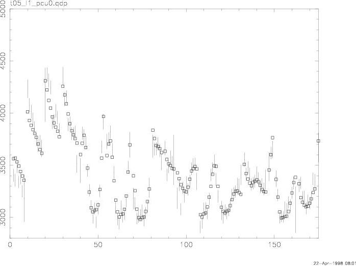
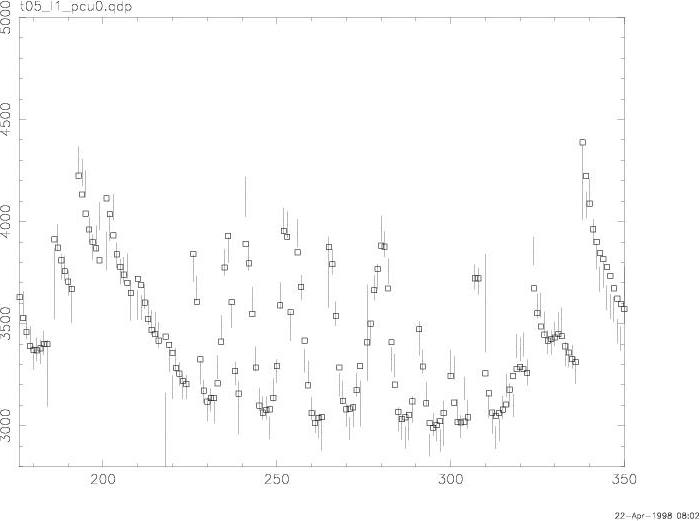
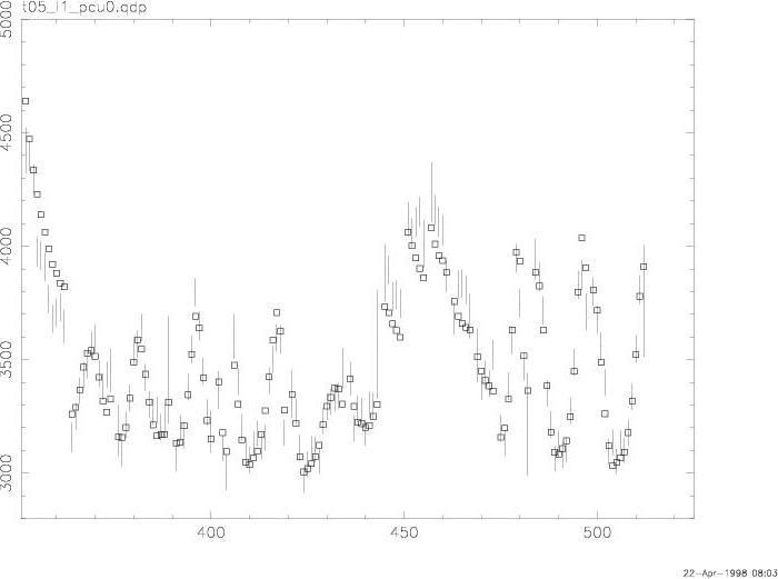
Data with +/- 1 sigma errors (vertical lines) and the model (squares) is shown for Pcu0 L1 in figures
1, 2, and 3. Time is not shown
here as the data is taken from several distinct times spread over more than a year. The x-axis is
instead just a running number for successive points. When the time between adjacent points is
greater than 256 seconds, I have inserted a blank point (without distinguishing whether the gap
is due to a brief occult or several weeks in length).
This is typical of the several tiome series
studied; correlations which describe the remaining scatter in the data are not yet identified.
It is easy to demonstrate the the worst fits are in the regions just after the SAA. For the example
illustrated above, the reduced chisq is 2.16 (210 points) for the subset of points that occur
between 30 and 60 minutes from the peak of an SAA and 1.45 (253 points) for the points that occur
more than 60 minutes from an SAA peak. This set happens to have the largest difference, but is
generally significant on all layers.
April 23, 1998
McIlwain L is globally < 1.7 for the data set illustrated above. There is no obvious correlation with the
residuals.
A model which includes a term proportion to the Vx rate seems to offer significant improvement, although
this can only be demonstrated for the entire layer, and not for any 25 channel subset.
April 24, 1998
Figure 4 shows the distribution of (data-prediction)/error for PCU 0, L1,
summed over all channels and 256 seconds. The width of this distribution (expected to be 1 in the
absence of systematics) is 1.23; the mean is 0.03 (or ~0.007 cs), believed to be consistent with
zero (needs to be compared to other data sets and data sets with more points).
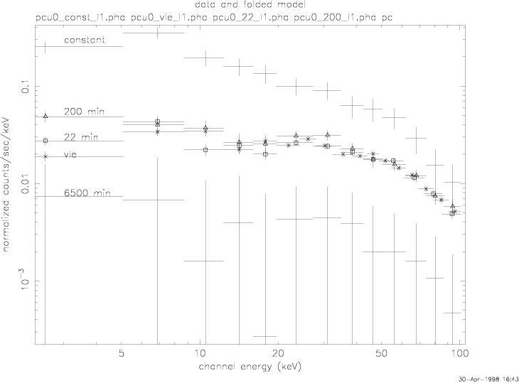
The relative contributions to figures 1,2, and 3 are shown in 5. The two most important terms (measured by total rate) are always the constant and VLE related terms. The short and medium time constants are important in the SAA orbits, and the long time constant term is the least variable.
April 27, 1998
Deconvolving the terms:
Figure 5 suggests how to separate the spectra for 5 different
contributing terms. During periods where the short and medium time constant activation
terms are low, the vle related term varies quite a bit. I defined two sets of time intervals
with the following criteria:
Medium_time_const < 100 AND VLE_related_rate > 900
Medium_time_const < 100 AND VLE_related_rate < 900
These two conditions select 115 and 121 (out of a total of 463) bins in the example I
have been illustrating. Extracting the data in these two intervals and differencing
gives the spectrum of the VLE related count rate. We have made two assumptions:
the activation related contributions to the two extractions are essentially similar;
the VLE related count rate has a constant spectrum and an amplitude which depends only
on the VLE rate.
The first assumption should be OK since the activation is selected to be low, and the
VLE variations are fast compared to the one time constant (the medium one) which might
vary significantly over this period. The second assumption will have to be tested
(by the consistency of our method or other means).
The short time constant term can be similarly estimated, so long as we select periods
where this is important, and the other terms are not too variable. The conditions
Medium_time_const_rate > 200 AND (index < 60 OR INDEX > 140) AND Short_time_const_rate > 150
Medium_time_const_rate > 200 AND (index < 60 OR INDEX > 140) AND Short_time_const_rate < 150
select 66 and 89 intervals. Doing better than this will require a larger data set.
Assumptions similar to those above apply.
The longer time constant terms cannot be estimated quite so easily, as there is
no possible selection that doesn't obviously violate the assumption that other rates
are not varying. Therefore, we select periods of high and low contribution
due to the medium time constant term, and correct the resulting spectra for
the assumed contribution of short time constant and VLE related terms. The criteria
to select the intervals are
Medium_time_const_rate > 300
Medium_time_const_rate < 100
which selects 135 and 236 points.
Estimating the longest time constant spectrum is similar, except that we correct for
the suitable normalized contribution of VLE, short and medium time constant terms. The
selection criteria were
Long_time_constant_rate > 260
Long_time_constant_rate < 240
which selects 152 and 169 bins.
The four derived spectra are shown in
6. There is a clear need for more statistical precision
for the 6500 sec spectrum (which has suffered the most subtractions, and has the
largest error bars)
April 30.
A larger data set has been fit to a model where the particle rate is scaled by the sum of the Vx counts (i.e. VxLCntPcu0 + VxHCntPcu0 + VxLVxHCntPcu0 ) plus three time constants as before. The data includes all the data from 20801-01, 20801-03, 20801-04, and 20801-05 (i.e. 4 different directions on the sky; the first layer may have extra unmodelled chi-squared due to cosmic fluctuations). The summaries of the fits are (note that B scales a different parameter than above)
          chi-sq     A                           B                           C_1                       tau_1                        C_2                        tau_2                       C_3                         tau_3
Pcu 0 L1   1.863  1.7681E+03 +/-  1.8208E+01  6.0736E-02 +/-  4.1613E-04  1.7336E-03 +/-  4.4236E-05  2.2000E+01 +/-  0.0000E+00  2.5767E-04 +/-  4.2794E-06  2.2000E+02 +/-  0.0000E+00  5.6617E-06 +/-  7.5723E-07  6.5000E+03 +/-
Pcu 0 L2   1.527  8.5856E+02 +/-  1.3704E+01  3.9199E-02 +/-  3.1428E-04  9.4301E-04 +/-  3.3403E-05  2.2000E+01 +/-  0.0000E+00  1.7036E-04 +/-  3.2270E-06  2.2000E+02 +/-  0.0000E+00  4.4379E-06 +/-  5.6975E-07  6.5000E+03 +/-
Pcu 0 L3   1.501  7.8881E+02 +/-  1.3541E+01  4.0543E-02 +/-  3.1098E-04  8.5424E-04 +/-  3.2875E-05  2.2000E+01 +/-  0.0000E+00  1.7023E-04 +/-  3.1807E-06  2.2000E+02 +/-  0.0000E+00  4.1226E-06 +/-  5.6228E-07  6.5000E+03 +/-  0.0000E+00
Pcu 1 L1   1.949  1.8523E+03 +/-  1.8564E+01  6.0730E-02 +/-  4.2041E-04  1.7380E-03 +/-  4.4749E-05  2.2000E+01 +/-  0.0000E+00  2.4761E-04 +/-  4.3357E-06  2.2000E+02 +/-  0.0000E+00  5.2934E-06 +/-  7.6895E-07  6.5000E+03 +/-  0.0000E+00
Pcu 1 L2   1.474  9.1918E+02 +/-  1.4128E+01  3.9695E-02 +/-  3.2087E-04  8.8506E-04 +/-  3.4154E-05  2.2000E+01 +/-  0.0000E+00  1.7042E-04 +/-  3.3049E-06  2.2000E+02 +/-  0.0000E+00  4.9019E-06 +/-  5.8473E-07  6.5000E+03 +/-  0.0000E+00
Pcu 1 L3   1.425  8.6663E+02 +/-  1.4016E+01  4.0615E-02 +/-  3.1908E-04  9.3434E-04 +/-  3.3870E-05  2.2000E+01 +/-  0.0000E+00  1.6013E-04 +/-  3.2753E-06  2.2000E+02 +/-  0.0000E+00  5.0392E-06 +/-  5.7979E-07  6.5000E+03 +/-  0.0000E+00
Pcu 2 L1   1.924  1.8765E+03 +/-  1.8624E+01  6.0020E-02 +/-  4.1942E-04  1.8318E-03 +/-  4.5166E-05  2.2000E+01 +/-  0.0000E+00  2.5392E-04 +/-  4.3677E-06  2.2000E+02 +/-  0.0000E+00  7.1974E-06 +/-  7.7358E-07  6.5000E+03 +/-  0.0000E+00
Pcu 2 L2   1.545  9.6594E+02 +/-  1.4051E+01  3.8215E-02 +/-  3.1711E-04  9.0063E-04 +/-  3.4124E-05  2.2000E+01 +/-  0.0000E+00  1.7239E-04 +/-  3.3019E-06  2.2000E+02 +/-  0.0000E+00  4.0765E-06 +/-  5.8311E-07  6.5000E+03 +/-  0.0000E+00
Pcu 2 L3   1.509  9.1762E+02 +/-  1.4058E+01  4.1785E-02 +/-  3.1828E-04  8.0217E-04 +/-  3.3927E-05  2.2000E+01 +/-  0.0000E+00  1.6376E-04 +/-  3.2874E-06  2.2000E+02 +/-  0.0000E+00  2.8368E-06 +/-  5.8329E-07  6.5000E+03 +/-  0.0000E+00  0.0000E+00 +/-  0.0000E+00  0.0000E+00 +/-  0.0000E+00
The 5 spectra are shown in 7. Application of these
spectra to reproducing the data is, naturally, the next step.
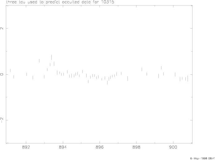
May 6, 1998
Today I compare the results of predicting the background with the 3 time constant
method and the layer 3 method. The data set is ~17 days of the P10315 observation
(Nandra PI). Data is selected for 3 PCU, layer 1, 2-10 keV. Initially background
estimates are done on 256 second timescales, although I have averaged 10 such intervals
for display purposes. I have determined a free parameter which is the offset between
blank sky and earth (deemed not interesting for this comparison, although we
can eventually make a global determination and investigate whether the dark earth
is constant).
Figure 8 shows the results using the three time constant
method. The results are encouraging, although there is a period near day 893 that fails.
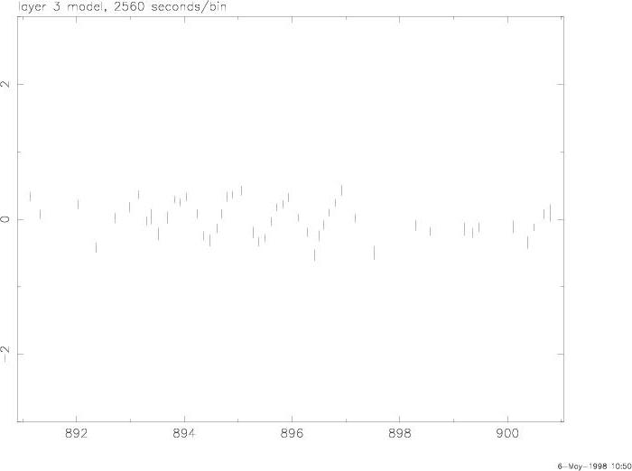
Figure 9 shows similar results for the layer 3 prediction.
There is no failure near day 893, but there is a suggestion of a daily variation from
day 892 to 898. The overall systematic variation (for this data set) is worse for the
layer 3 prediction. For both data sets, the background was estimated independently for
each of the three detectors and then summed.