\(T\) - \(\log\xi\) curves

Here we compare heating and cooling rates as function of temperature \(T\) and ionization parameter \(\log\xi\). First we create a grid of temperatures and ionization parameters.

>>> import numpy as np
>>> import os
>>> import matplotlib.pyplot as plt
>>> from astropy.io import fits

>>> nt = 31 # Number of temperature steps
>>> nlxi = 31 # Number of logxi steps
>>> lxi = np.linspace(-1, 5, num=nlxi) # Step logxi  from 1 to 5
>>> t =  np.logspace(0, 4, num=nt) # Temperature from 1E0 to 1E4
>>> httot = np.zeros((nt, nlxi))
>>> cltot = np.zeros((nt, nlxi))

Then we loop over this grid and run xstar for each combination of \(T\) and \(\log\xi\). This can be very time-consuming depending on the ranges and stepsize of the \(T\)- \(\log\xi\) grid. Note that niter is set to 0 in order to keep the temperature fixed at its input value. The total heating and cooling rates can be read from the ion abundance output file.

>>> for ii in range(0, nt):
...       for jj in range(0, nlxi):
...         xstcmd = "xstar cfrac=1  pressure=0.03 density=1E12 trad=-1. spectrum='pow' rlrad38=1E6 column=1E10 nsteps=3 niter=0 lwrite=0 lprint=0 lstep=0 npass=1 lcpres=0 emult=0.5 taumax=5. xeemin=0.1 critf=1E-8 vturbi=300 radexp=0 ncn2=999 modelname='t-xi' abundtbl='xdef' loopcontrol=0 rlogxi={rlogxi} temperature={temp:.2E}".format(rlogxi = lxi[jj], temp = t[ii])
...         os.system(xstcmd) # Run xstar
...         hdul = fits.open('xout_abund1.fits')
...         httot[ii,jj] = hdul[3].data['total'][0] # Read total heating rate
...         cltot[ii,jj] = hdul[4].data['total'][0] # Read total cooling rate
...         hdul.close()
...         os.system("rm xout_abund1.fits  xout_cont1.fits  xout_lines1.fits  xout_rrc1.fits  xout_spect1.fits  xout_step.log") # Clean up

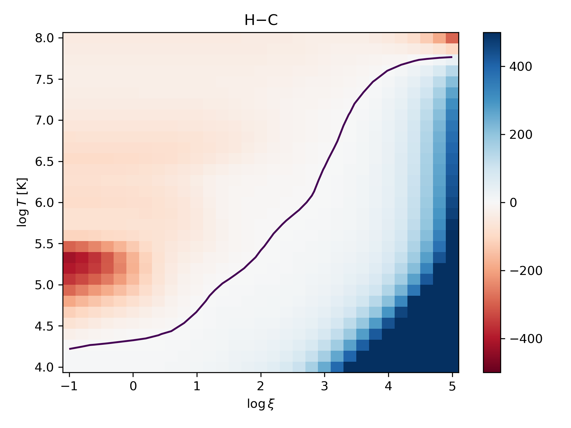
Finally we plot heating minus cooling as a 2D map and draw a contour of thermal equilibrium.

>>> hmc=httot-cltot
>>> fig, ax = plt.subplots(1, 1)
>>> c = ax.pcolor(lxi,np.log10(t)+4, hmc, cmap='RdBu',vmin=-500, vmax=500)
>>> ax.set_title('H$-$C')
>>> ax.set_ylabel("$\\log T$ [K]")
>>> ax.set_xlabel("$\\log\\xi$")
>>> ax.contour(lxi,np.log10(t)+4, hmc, levels=[0.0])
>>> fig.colorbar(c, ax=ax)
>>> fig.tight_layout()
>>> plt.show()