

THE XMM-NEWTON ABC GUIDE, STREAMLINED
EPIC (IMAGING mode), SAS GUI
Contents
Prepare the Data
Reprocess the Data
Introduction to xmmselect
Apply Standard Filters
Make a Light Curve
Apply Time Filters
Making an Image and Source Detection
Make an Exposure Map
Extract the Source and Background Spectra
Check for Pile Up
My Observation is Piled Up! Now What?
Determine the Spectrum Extraction Areas
Create the Photon Redistribution Matrix (RMF) and Ancillary File (ARF)
Prepare the Data
Please note that the two tasks in this section (cifbuild and odfingest) must be run in the ODF directory. These are the only tasks with that requirement, and after this section, we will work exclusively in our reprocessing directory.Many SAS tasks require calibration information from the Calibration Access Layer (CAL). Relevant files are accessed from the set of Current Calibration File (CCF) data using a CCF Index File (CIF).
To make the ccf.cif file, first make sure the environment variables are set:
   cd ODF
   setenv SAS_ODF /full/path/to/ODF/directory/
   setenv SAS_ODFPATH /full/path/to/ODF/directory/
Next, call cifbuild from the SAS GUI. A window with the parameter options will appear; the defaults should be fine, so just click "Run".
To use the updated CIF file in further processing, you will need to reset the environment variable SAS_CCF:
setenv SAS_CCF /full/path/to/ODF/ccf.cifThe task odfingest extends the Observation Data File (ODF) summary file with data extracted from the instrument housekeeping data files and the calibration database. It is only necessary to run it once on any dataset, and will cause problems if it is run a second time. If for some reason odfingest must be rerun, you must first delete the earlier file it produced. This file largely follows the standard XMM naming convention, but has SUM.SAS appended to it. After running odfingest, you will need to reset the environment variable SAS_ODF to its output file. To run odfingest and reset environment variable, call odfingest from the SAS GUI. As before, a pop-up window with the parameter options will appear; the defaults should be fine, so just click "Run". (It is safe to ignore the warnings.)
To change the environmental variable, type
setenv SAS_ODF /full/path/to/ODF/full_name_of_*SUM.SASYou will likely find it useful to alias these environment variable resets in your login shell (.cshrc, .bashrc, etc.).
Reprocess the Data
To reprocess the data, make a new working directory and from it, call emproc for MOS data, and epproc for PN data.cd .. mkdir PROC cd PROCThen, close and re-open the SAS GUI, so that it will place the output files in the new directory, and call the pipeline tasks. The defaults are fine for most observations, so just click "Run". (It is safe to ignore the warnings.)
By default, none of these tasks keep any intermediate files they generate. Emproc and epproc designate their output event files with "ImagingEvts.ds". It is convenient to rename them something easy to type, for instance:
cp 0070_0123700101_EMOS1_S001_ImagingEvts.ds mos1.fits
Introduction to xmmselect
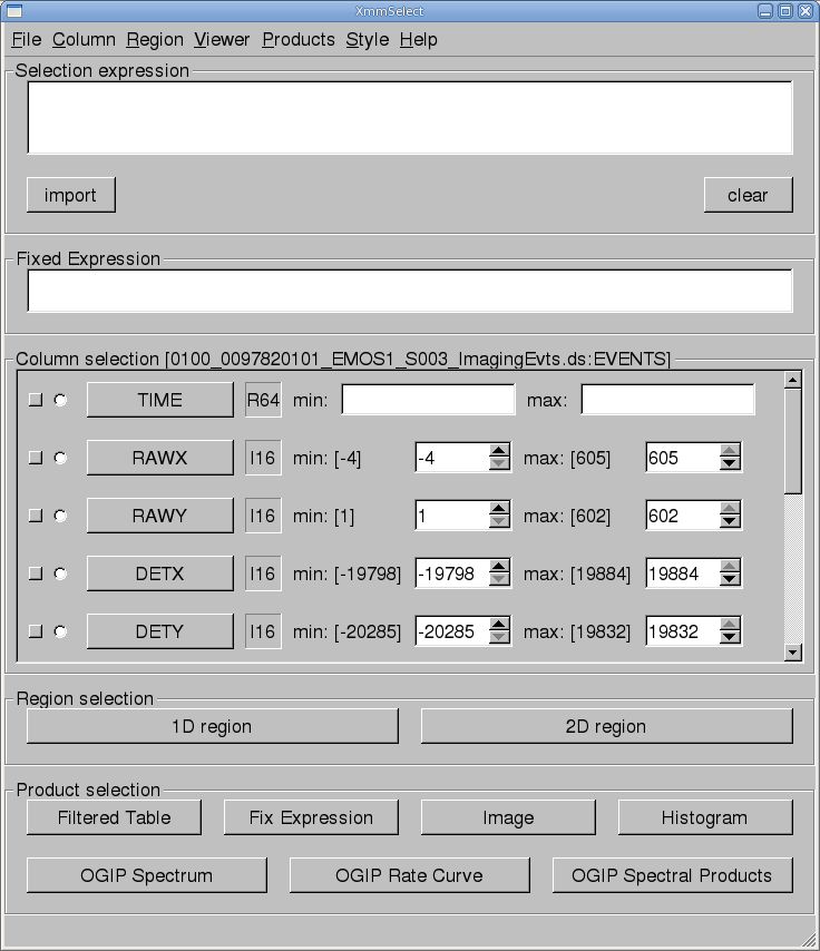
The task xmmselect is used for many procedures in the GUI. Like all tasks, it can easily be invoked by starting to type the name and pressing enter when it is highlighted.When xmmselect is invoked a dialog box will first appear requesting a file name. You can either use the browser button or just type the file name in the entry area, "mos1.fits:EVENTS" in this case. To use the browser, select the file folder icon; this will bring up a second window for the file selection. Choose the desired event file, then the "EVENTS" extension in the right-hand column, and click "OK". The directory window will then disappear and you can click "Run" on the selection window.
When the file name has been submitted the xmmselect GUI will appear, along with a dialog box offering to display the selection expression; this is shown in Figure 1. The selection expression will include the filtering done to this point on the event file, which for the pipeline processing includes for the most part CCD and GTI selections.
Different event files can be loaded into xmmselect by going to "File -> New Table".
Apply Standard Filters
The filtering expressions for the MOS and PN are:
(PATTERN <= 12)&&(PI in [200:12000])&&#XMMEA_EM
and
(PATTERN <= 4)&&(PI in [200:15000])&&#XMMEA_EP
If you are going to extract a spectrum from the PN data, you will need the most stringent filters in order to get a high-quality spectrum:
(PATTERN <= 4)&&(PI in [200:15000])&&#XMMEA_EP&&(FLAG == 0)
For the MOS, the standard filters should be appropriate for most cases.
The first two expressions will select good events with PATTERN in the 0 to 12 range. The PATTERN value is similar the GRADE selection for ASCA data, and is related to the number and pattern of the CCD pixels triggered for a given event.The PATTERN assignments are: single pixel events: PATTERN == 0, double pixel events: PATTERN in [1:4], triple and quadruple events: PATTERN in [5:12].
The second keyword in the expressions, PI, selects the preferred pulse height of the event; for the MOS, this should be between 200 and 12000 eV. For the PN, this should be between 200 and 15000 eV. This should clean up the image significantly with most of the rest of the obvious contamination due to low pulse height events. Setting the lower PI channel limit somewhat higher (e.g., to 300 eV) will eliminate much of the rest.
Finally, the #XMMEA_EM (#XMMEA_EP for the PN) filter provides a canned screening set of FLAG values for the event. (The FLAG value provides a bit encoding of various event conditions, e.g., near hot pixels or outside of the field of view.) Setting FLAG == 0 in the selection expression provides the most conservative screening criteria and should always be used when serious spectral analysis is to be done on the PN. It typically is not necessary for the MOS.
To filter the data using xmmselect,
- Enter the filtering criteria in the "Selection Expression" area at the top of the xmmselect window:
(PATTERN <= 12)&&(PI in [200:12000])&&#XMMEA_EM
- Click on the "Filtered Table" box at the lower left of the xmmselect GUI.
- Change the evselect filteredset parameter, the output file name, to something useful, e.g., mos1_filt.fits.
- Click "Run".
Make a Light Curve
Sometimes, it is necessary to use filters on time in addition to those mentioned
above. This is because of soft proton background flaring, which can have count rates
of 100 counts/sec or higher across the entire bandpass.
It should be noted that the amount of flaring that needs to be removed depends in
part on the object observed; a faint, extended object will be more affected than
a very bright X-ray source.
To determine if our observation is affected by background flaring, we can make a light curve by calling xmmselect and loading the event file as shown above. Then,
- Check the round box to the left of the "Time" entry.
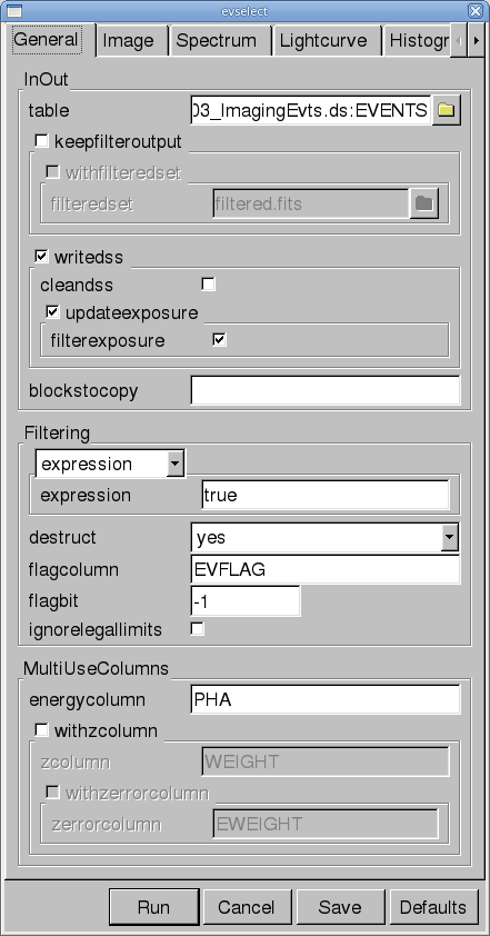
- Click on the "OGIP Rate Curve" button near the bottom of the page. This brings up the evselect GUI (see Figure 2).
- Click on the "Lightcurve" tab and change the "timebinsize" to a reasonable amount, e.g. 10 or 100 s. In the "rateset" textbox, enter the name of the output file, for example, mos1_ltcrv.fits.
- Click on the "Run" button at the lower left corner of the evselect GUI.
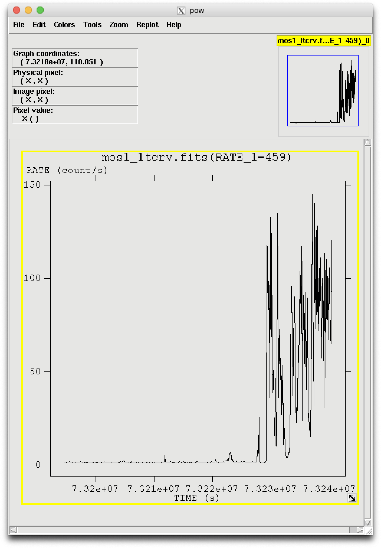
The output file can be viewed by using fv and is shown in Figure 3.
fv mos1_ltcrv.fits &
Apply Time Filters
Taking a look at the light curve, we can see that there is a very large flare toward the end of the observation and two much smaller ones in the middle of the exposure.
There are several ways to filter an event file: on TIME, with an explicit reference to the TIME parameter in the filtering expression or by creating a secondary Good Time Interval (GTI) file, or on RATE, which requires making a new GTI file. New GTI files are easily made with the task tabgtigen or gtibuild. These are discussed in detail below. Any of these methods will produce a cleaned file, so which one to use is a matter of the user's preference
Filter on RATE With tabgtigen
Examining the light curve shows us that during non-flare times, the count rate
is quite low, about 1.3 ct/s, with a small increase at 7.3223e7 seconds to about
6 ct/s. We can use that to generate the GTI file by calling tabgtigen
from the SAS GUI and loading the light curve's RATE table as the input table. Then,
- Edit the output file name, the gtiset parameter; here, we will use gtiset.fits.
- Enter the filtering expression, (RATE <= 6).
- Click "Run".
The new GTI file can be applied with xmmselect by calling that task and loading the event file mos1_filt.fits and its EVENTS extension. Then,
- In the "Selection Expression" box, type GTI(gtiset.fits,TIME).
- Click on the "Filtered Table" box at the lower left of the xmmselect GUI.
- Change the evselect filteredset parameter, the output file name, to something useful; here, we will use mos1_filt_time.fits.
- Click "Run".
Filter on TIME With tabgtigen
Alternatively, we could have chosen to make a new GTI file by noting the times of
the flaring in the light curve and using that as a filtering parameter. The big flare
starts around 7.32276e7 s, and the smaller ones are at 7.32119e7 s and 7.32205e7 s.
The expression to remove these would be (TIME <= 73227600)&&!(TIME IN
[7.32118e7:7.3212e7])&&(TIME IN [7.32204e7:7.32206e7]).
The syntax &&(TIME < 73227600) includes only events with times
less than 73227600, and the "!" symbol stands for the logical "not", so use
&&!(TIME in [7.32118e7:7.3212e7]) to exclude events in that time
interval. To use these filtering parameters, call tabgtigen from the SAS GUI
and load the light curve's RATE extention. Then,
- Edit the output file name, the gtiset parameter; here, we will use gtiset.fits.
- Enter the filtering expression, (TIME <= 73227600)&&!(TIME IN [7.32118e7:7.3212e7])&&!(TIME IN [7.32204e7:7.32206e7])
- Click "Run".
The new GTI file can be applied with xmmselect. With the mos1_filt.fits event file loaded,
- In the "Selection Expression" box, type GTI(gtiset.fits,TIME).
- Click on the "Filtered Table" box at the lower left of the xmmselect GUI.
- Change the evselect filteredset parameter, the output file name, to something useful; here, we will use mos1_filt_time.fits.
- Click "Run".
Filter on TIME With gtibuild
This method requires a text file as input. In the first two columns, enter the start and
end times (in seconds) that you are interested in, and in the third column, indicate with
either a + or - sign whether that region should be kept or removed. Each good (or bad)
time interval should get its own line, with any optional comments preceeded by a "#". In
the example case, we would write in our ASCII file (named gti.txt):
   0 73227600 +          # Good time from the start of the observation...
   7.32118e7 7.3212e7 -  # but without a small flare here,
   7.32204e7 7.32206e7 - # and here.
and proceed to gtibuild. Invoke the task, then
- Enter the name of the text file as the file parameter.
- Enter the output name in the table parameter; we will use gtiset.fits.
- Click "Run".
Filter on TIME by Explicit Reference
Finally, we could have chosen to forgo using tabgtigen or gtibuild altogether, and
simply filtered on TIME with the
standard filtering expression. In that case, the full filtering expression would be:
   (PATTERN <= 12) && (PI in [200:12000]) && #XMMEA_EM &&
      (TIME <= 73227600) &&! (TIME IN [7.32118e7:7.3212e7]) &&! (TIME IN [7.32204e7:7.32206e7])
This expression can then be used to
filter the original event file, or only the times can be used to filter the
file that has already had the standard filters applied. To do this, load the
filtered event file mos_filt.fits in xmmselect by going to
"File -> New Table" at the top of the window, and loading it as shown
above. Then,
- Enter the filtering criteria in the "Selection Expression" area at the top
of the xmmselect GUI:
(TIME <= 73227600) &&! (TIME IN [7.32118e7:7.3212e7]) &&! (TIME IN [7.32204e7:7.32206e7]) - Click on the "Filtered Table" box at the lower left of the window.
- Change the evselect filteredset parameter, the output file name, to something useful, e.g., mos1_filt_time.fits.
- Click "Run".
Source Detection
The edetect_chain task does nearly all the work involved with EPIC source detection. It can process up to three intruments (both MOS cameras and the PN) with up to five images in different energy bands simultaneously. All images must have identical binning and WCS keywords. For this example, we will perform source detection on MOS1 images in two bands (``soft'' X-rays with energies between 300 and 2000 eV, and ``hard'' X-rays, with energies between 2000 and 10000 eV) using the filtered event files produced here. Edetect_chain has many parameters that users might want to edit, such as detection likelihood threshold; more information about them can be found here.
We will start by generating some files that edetect_chain needs: an attitude file and images of the sources in the desired energy bands.
First, make the attitude file by calling atthkgen in the SAS GUI. Then,
- Verify that timestep is set to 1. Set the atthkset keyword to the desired output file name, for example, attitude.fits.
- Click "Run".
Next, the images. We can choose either to bin to a certain image size (by setting the imagebinning parameter to imageSize and specifying values for ximagesize and yimagesize; the default values makes a 600x600 pixel image), or we can set the bin size directly (by setting imagebinning to binSize and specifying values for ximagebinsize and yimagebinsize).
In order to select a reasonable binsize, we need to know a little about the detectors themselves. The pixels of the MOS and PN cameras correspond to 1.1'' and 4.1'' on the sky, respectively, but photons incident on the detector have their positions randomized within these pixels into "virtual pixels" of size 0.05''. So, if we want image pixels that correspond to 1.1'' (or 4.1'') we need a bin size of 22 (or 82).
In addition to making images in soft and hard bands, we'll also make an image that includes both bands, for display purposes.
Call evselect in the SAS GUI, then
- In the "General" tab, set the "Table" parameter to the MOS1 event file name,
mos1_filt_time.fits. Confirm that "Filtertype" is set to "expression",
and in the "Expression" text area, type
(FLAG == 0)&&(PI in [300:2000])
- In the "Image" tab, check the withimageset box, and enter the desired output image name; we will use mos1-s.fits. Set xcolumn to X and ycolumn to Y. Set Binning to binSize, ximagebinsize to 22, and yimagebinsize to 22.
- Click "Run".
Follow the same procedure to make the hard X-ray image, changing the output name to mos1-h.fits and the filtering expression to (FLAG == 0)&&(PI in [2000:10000]). For our combined band image, we'll set the output name to mos1-all.fits and the filtering expression to (FLAG == 0)&&(PI in [300:10000]).
Now we can run edetect_chain. Call the task, and then
- In the "0" tab, in the imagesets text area, enter the image names separated by a space: mos1-s.fits mos1-h.fits. In the eventsets area, enter the name of the event file: mos1_filt_time.fits. In the attitudeset area, enter the name of the attitude file made by atthkgen, attitude.fits. Set the pimin keyword to the minimum PI values (in eV) for the input images, separated by a space: 300 2000, and do similar for the maximum values for pimax 2000 10000. Set the likemin parameter to 10, witheexpmap to yes. Set the energy conversion factors,ecf, to appropriate values for the two bands, separated by white space; here we will use 0.878 0.220.
- In the "1" tab, set eboxl_list to eboxlist_l.fits and eboxm_list to eboxlist_m.fits.
- In the "2" tab, set esp_withootset to no and eml_list to emllist.fits.
- Click "Run".
The energy conversion factors (ECFs) convert the source count rates into fluxes. The ECFs for each detector and energy band depend on the pattern selection and filter used during the observation. For more information, please consult the 3XMM Catalogue User Guide. Those used here are derived from PIMMS using the flux in the 0.1-10.0 keV band, a source power-law index of 1.9, an absorption of 0.5×1020cm-2.
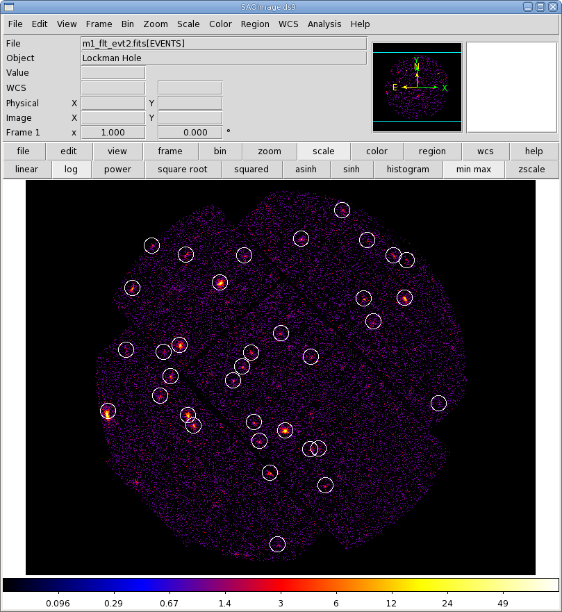
We can display the results of eboxdetect using srcdisplay and produce a region file for the sources. Call srcdisplay, and then
- Set boxlistset to emllist.fits. Confirm that withimageset is checked, and set imageset to an image name; we will use the soft band image, mos1-s.fits. Check withregionfile, and set regionfile to regionfile.txt. Confirm that sourceradius is set to 0.01.
- Click "Run".
Figure 4 shows the MOS1 event file overlayed with the detected sources.
Make an Exposure Map
Prior to making an exposure map, you will need to make an image in the energy band you are interested in. You will also need the attitude file from atthkgen. Let's say that we're interested in the 1-2 keV band; we can use the attitude file that we made before. To make the image, call evselect, then
- In the "General" tab, set the "Table" parameter to the MOS1 event file name, mos1_filt_time.fits. Confirm that "Filtertype" is set to "expression", and in the "Expression" text area, enter (PI in [1000:2000]).
- In the "Image" tab, check the withimageset box, and enter the desired output image name; we will use mos1_1-2keV.fits. Set xcolumn to X and ycolumn to Y. Set Binning to binSize, ximagebinsize to 22, and yimagebinsize to 22
- Click "Run".
Then, call eexpmap and
- Set imageset to mos1_1-2keV.fits and set the attitudeset parameter to attitude.fits. By the eventset parameter, enter the event file, mos1_filt_time.fits. Enter an output file name in expimageset; we will use mos1_expmap_1-2keV.fits. In pimin, enter the lower PI value from the image, 1000. Do the same for the higher PI value in the parameter pimax, 2000.
- Click "Run".
Extract the Source and Background Spectra
Throughout the following, please keep in mind that some parameters are instrument-dependent. The parameter specchannelmax should be set to 11999 for the MOS, or 20479 for the PN. Also, for the PN, the most stringent filters, (FLAG==0)&&(PATTERN<=4), must be included in the expression to get a high-quality spectrum.For the MOS, the standard filters should be appropriate for many cases, though there are some instances where tightening the selection requirements might be needed. For example, if obtaining the best possible spectral resolution is critical to your work, and the corresponding loss of counts is not important, only the single pixel events should be selected (PATTERN==0). If your observation is of a bright source, you again might want to select only the single pixel events to mitigate pile up.
There is more than one way to do this; for this example, we will use xmmselect. Load the filtered event file into xmmselect. Then,
- Make an image by checking the square boxes to the left of the "X" and "Y" entries. Click the "Image" button near the bottom of the page. This brings up the evselect GUI.
- In the "Image" tab, enter the name of the output file in the imageset box; we will use mos1_image.fits. Different binnings and other selections can be invoked, but the default settings are reasonable for a basic image.
- Click the "Run" button on the lower left corner of the evselect GUI. The image will be displayed automatically in a ds9 window.
- Click on the object whose spectrum you wish to extract. This will produce an extraction region, centered on the object. The circle's radius can be changed by clicking on it. Adjust the size and position of the circle until you are satisfied with the extraction region. We will use the source at x=26188.5 and y=22816.
- Click on "2D Region" in the xmmselect GUI. This transfers the region information into the "Selection Expression" text area, for example, ((X,Y) IN circle(26188.5,22816,300)). Click the round button next the PI column on the xmmselect GUI, then click on "OGIP Spectrum". This will bring up the evselect GUI.
- In the "General" tab, check keepfilteroutput and withfilteredset. In the filteredset box, enter the name of the event file output. We will use mos1_filtered.fits.
- Select the "Spectrum" tab of the evselect GUI to set the file name and binning parameters for the spectrum. Confirm that withspectrumset is checked. Set spectrumset to the desired output name, in this case, mos1_pi.fits. Confirm that withspecranges is checked. Confirm that specchannelmin is 0 and specchannelmax is 11999 for the MOS, or 20479 for the PN.
- Click "Run".
The background spectrum can be extracted following the same method, setting the region to an annulus around the source: ((X,Y) in CIRCLE(26188.5,22816.5,1500))&&!((X,Y) in CIRCLE(26188.5,22816.5,500)). We will call the filtered event file bkg_filtered.fits and the output spectrum bkg_pi.fits.
Check for Pile Up
Depending on how bright the source is and what modes the EPIC detectors are in, event pile up may be a problem. Pile up occurs when a source is so bright that incoming X-rays strike two neighboring pixels or the same pixel in the CCD more than once in a read-out cycle. In such cases the energies of the two events are in effect added together to form one event. If this happens sufficiently often, 1) the spectrum will appear to be harder than it actually is, and 2) the count rate will be underestimated, since multiple events will be undercounted. To check whether pile up may be a problem, use the SAS task epatplot. Heavily piled sources will be immediately obvious, as they will have a "hole" in the center of their image, but pile up is not always so conspicuous. Therefore, we recommend to always check for it.
Note that this procedure requires as input the event file created when the spectrum was made, not the usual time-filtered event file.
To check for pile up in our Lockman Hole example, invoke epatplot. Then,
- In the "0" tab, enter the name of the event file that was made when the spectrum was extracted, mos1_filtered.fits, in the set text box. We want to send the output to a ps file, so set useplotfile to yes, and enter the file name in the plotfile box. We will use mos1_epat.ps.
- In the "1" tab, set withbackgroundset to yes and enter the name of the event file that was made when the background spectrum was made, bkg_filtered.fits.
- Click "Run".
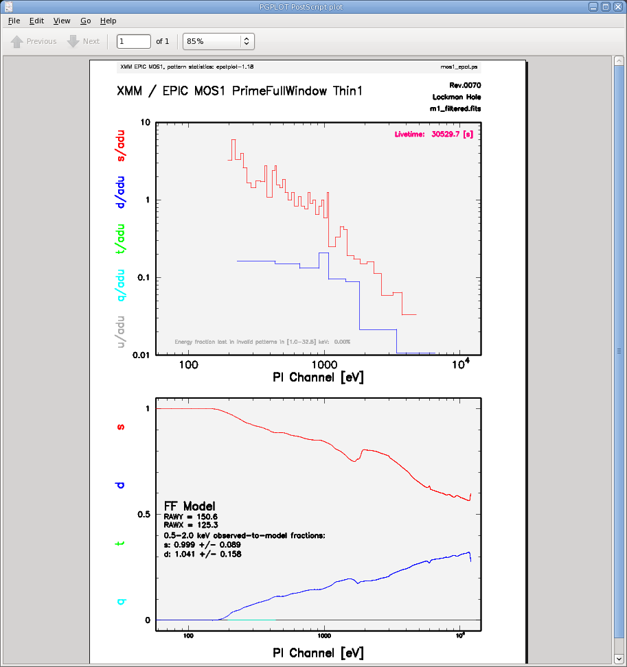
The output of epatplot is a postscript file, mos1_epat.ps, which may be viewed with viewers such as gv, containing two graphs describing the distribution of counts as a function of PI channel, as seen in Figure 5 (left).
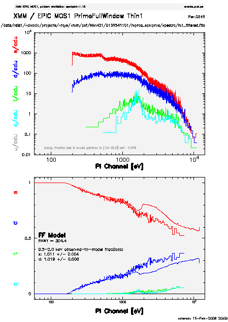
A few words about interpretting the plots are in order. The top is the distribution of counts versus PI channel for each pattern class (single, double, triple, quadruple), and the bottom is the expected pattern distribution (smooth lines) plotted over the observed distribution (histogram). The lower plot shows the model distributions for single and double events and the observed distributions. It also gives the ratio of observed-to-modeled events with 1-σ uncertainties for single and double pattern events over a given energy range. (The default is 0.5-2.0 keV; this can be changed with the pileupnumberenergyrange parameter.) If the data is not piled up, there will be good agreement between the modeled and observed single and double event pattern distributions. Also, the observed-to-modeled fractions for both singles and doubles in the specified energy range will be unity, within errors. In contrast, if the data is piled up, there will be clear divergence between the modeled and observed pattern distributions, and the observed-to-modeled fraction for singles will be less than 1.0, and for doubles, it will be greater than 1.0.
Finally, when examining the plots, it should noted that the observed-to-modeled fractions can be inaccurate. Therefore, the agreement between the modeled and observed single and double event pattern distributions should be the main factor in determining if an observation is affected by pile up or not.
The source used in our Lockman Hole example is too faint to provide reasonable statistics for epatplot and is far from being affected by pile up. For comparison, an example of a bright source (from a different observation) which is strongly affected by pileup is shown in Figure 5 (right). Note that the observed-to-model fraction for doubles is over 1.0, and there is severe divergence between the model and the observed pattern distribution.
|
My Observation is Piled Up! Now What?
If you're working with a different (much brighter) dataset that does show signs of pile up, there are a few ways to deal with it. First, using the region selection and event file filtering procedures demonstrated in earlier sections, you can excise the inner-most regions of a source (as they are the most heavily piled up), re-extract the spectrum, and continue your analysis on the excised event file. For this procedure, it is recommended that you take an iterative approach: remove an inner region, extract a spectrum, check with epatplot, and repeat, each time removing a slightly larger region, until the model and observed distribution functions agree. If you do this, be aware that removing too small a region with respect to the instrumental pixel size (1.1'' for the MOS, 4.1'' for the PN) can introduce systematic inaccuracies when calculating the source flux; these are less than 4%, and decrease to less than 1% when the excised region is more than 5 times the instrumental pixel half-size. In any case, be certain that the excised region is larger than the instrumental pixel size!
You can also use the event file filtering procedures to include only single pixel events (PATTERN==0), as these events are less sensitive to pile up than other patterns.
Determine the Spectrum Extraction Areas
Now that we are confident that our spectrum is not piled up, we can continue by finding the source and background region areas. This is done with the task backscale, which takes into account any bad pixels or chip gaps, and writes the result into the BACKSCAL keyword of the spectrum table. Alternatively, we can skip running backscale, and use a keyword in arfgen below. We will show both options for the curious.
To find the source extraction area explicitly, call backscale and then
- In the "Main" tab, enter the name of the spectrum, mos1_pi.fits.
- In the "Effects" tab, confirm that withbadpixcorr is checked, and enter the name of the event file in badpixlocation.
- Click "Run".
Follow the same steps to find the background spectrum area, changing the input spectrum file to bkg_pi.fits.
Create the Photon Redistribution Matrix (RMF) and Ancillary File (ARF)
Now that a source spectrum has been extracted, we need to reformat the detector response by making a redistribution matrix file (RMF) and ancillary response file (ARF).
To make the RMF, call rmfgen and then
- In the "main" tab, set rmfset to the output file name. We will use mos1_rmf.fits. Set the spectrumset parameter to the spectrum, mos1_pi.fits.
- Click "Run".
Now use the RMF, spectrum, and event file to make the ancillary file. Invoke arfgen, and then
- In the "main" tab, set arfset to the output file name. We will use mos1_arf.fits. Set the spectrumset parameter to the spectrum, mos1_pi.fits.
- In the "calibration" tab, set withrmfset to yes and rmfset to the RMF file, mos1_rmf.fits.
- In the "effects" tab, verify that withbadpixcorr is checked, and set badpixlocation to the event file, mos1_filt_time.fits.
- Click "Run".
If we had not run backscale, we could set a keyword in arfgen to find the region area. In addition to the steps above,
- In the "backscale" tab, set setbackscale to yes.
The spectrum can be fit using HEASoft or CIAO packages, as SAS does not include fitting software.
If you have any questions concerning XMM-Newton send e-mail to xmmhelp@lists.nasa.gov