

THE XMM-NEWTON ABC GUIDE, STREAMLINED
Approaches to Spectral Fitting and the Cash Statistic (cstat)
Before we get to fitting the spectrum, a few words are in order about different approaches to take.
Traditional thinking holds that for data sets of high signal-to-noise and low background, where counting statistics are within the Gaussian regime, an analysis using the default fitting scheme in Xspec and Sherpa (χ2-minimization) is appropriate. For low count rates (< 5 counts/bin), in the Poisson regime, χ2-minimization is no longer suitable, as the error per channel can dominate over the count rate. Since channels are weighted by the inverse-square of the errors during χ2 model fitting, channels with the lowest count rates are given overly-large weights in the Poisson regime. This leads to spectral continua that are fit incorrectly, with the model lying underneath the true continuum level.
The traditional way to increase the signal-to-noise of a data set is to rebin or group the channels, since, if channels are grouped in sufficiently large numbers, the combined signal-to-noise of the groups will jump into the Gaussian regime. However, this results in the loss of information. For example, sharp features like an absorption edge or emission line can be washed out. This is a particular problem for high resolution RGS data; even if count rates are large, much of the flux from these sources can be contained within emission lines, rather than the continuum. Consequently, even obtaining correct equivalent widths for such sources is non-trivial. Further, in the Poisson regime, the background spectrum cannot simply be subtracted, as is commonly done in the Gaussian regime, since this could result in negative counts. Therefore, for analysis of high resolution spectra, using the Cash statistic (cstat) on unbinned spectra has become standard practice; if an assessment of the background is necessary, the unbinned background spectrum is fitted simultaneously. Rebinning and using χ2 should be reserved for fast, preliminary analysis of spectra without sharp features, or for making plots for publication.
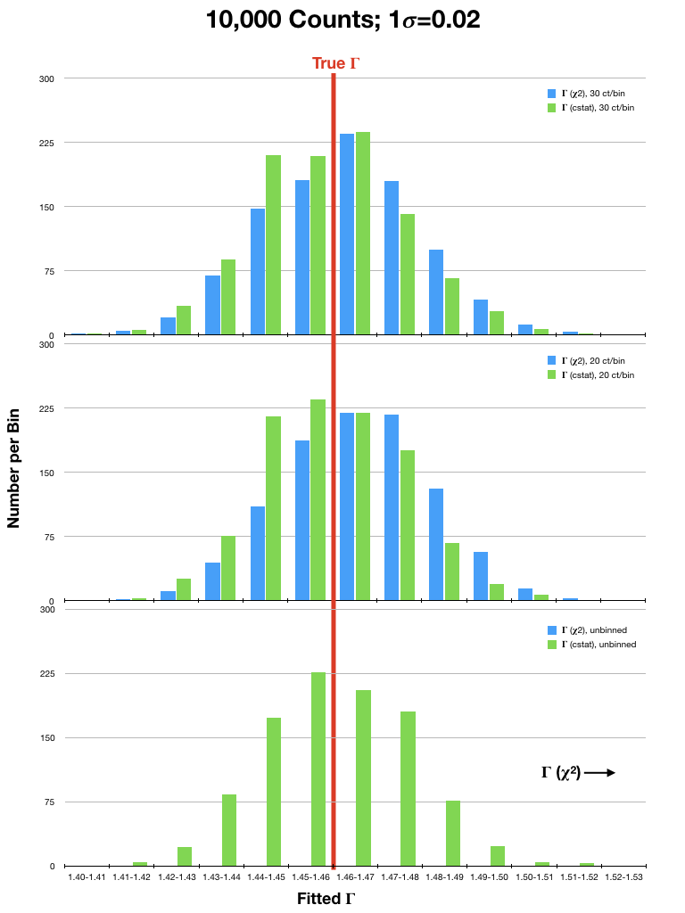
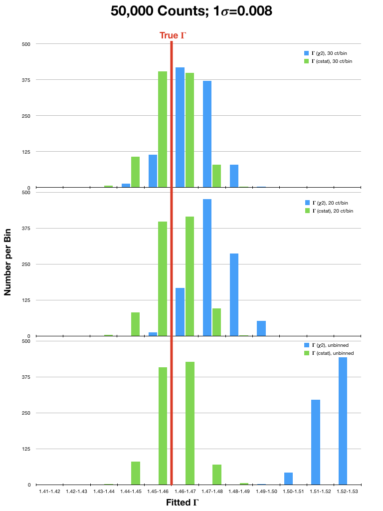
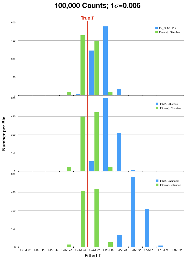
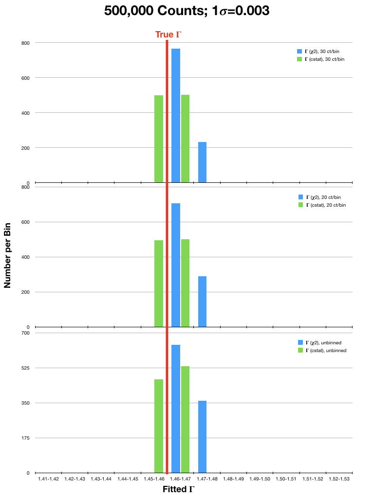
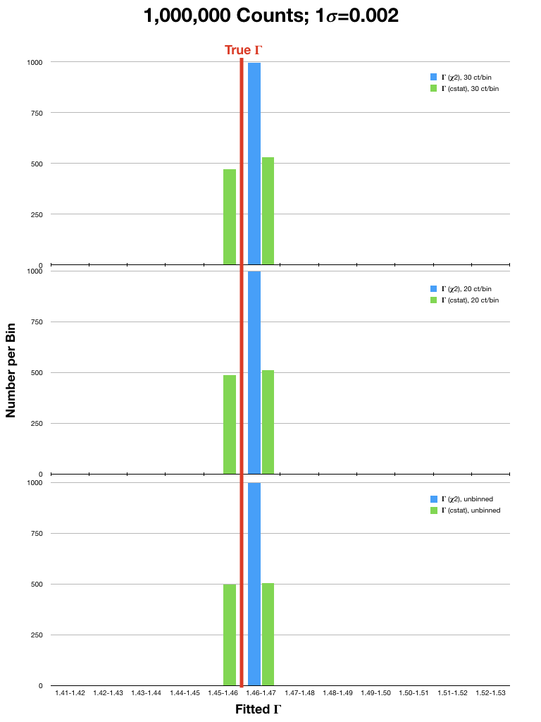
For analysis of (mostly smooth) low resolution spectra, which are typically in the high count regime, spectra are often rebinned and χ2 statistics are used. However, investigations into the validity of χ2 statistics in the high count regime have shown that they can still yield biased results. To illustrate this, we have run sets of simulations of an EPIC PN spectrum (a lightly absorbed power law with Γ=1.46) using a canned response file. In each simulation, the spectrum was either binned to 20 or 30 counts per bin, or not binned at all, and fitted with χ2 statistics with the Gehrels variance function and cstat. The simulations were run considering different source fluxes, with 104, 5x10⁴, 105, 5x10⁵, and 106 counts per spectrum over the range 0.3-15.0 keV. Each simulation was run 1,000 times. The resulting best-fit values of Γ were then compared to the true value. Plots of the results are in Fig. 1 (click on a plot for a larger image).
|
It can be seen that the Gehrels χ2 fits tended to find best-fit values of Γ that were 2- or 3-σ (or more!) higher than the true value, even in spectra with high fluxes. This is particularly true for the fits to spectra that were rebinned to only 20 counts/bin. In contrast, cstat was able to recover Γ with much better accuracy in both the high and low count regimes, regardless of binning. The difference in the accuracy of the results obtained with χ2 and cstat diminished only when the number of counts in the spectrum were very high (≥ 1 million). It is therefore recommended that users examine their data carefully before deciding which statistic and binning, if any, is appropriate for their spectra.
Optimization
The optimization method (i.e., the method used to find the minimum or maximum of a function) can also affect the accuracy of the fit. This is because a fitting function can have one or more local minima, and optimization methods can become stuck in a local minimum rather than finding the global minimum. A commonly used optimization method is Levenberg-Marquardt (LM); this is the default of many software packages. It has the benefit of being fast, but this comes at the price of being susceptible to getting pulled into local minima, especially if the initial values of the fitting parameters were far from their real values. Nelder-Mead is less susceptible to local minima, but it takes longer, and can get stuck going in circles around a minimum rather than converging to it like LM. Therefore, users might wish to use both methods to ensure that their fit is robust.A Word About XSpec
If fitting RGS data with XSpec, be sure you are running v11.1.0 or later. This is because RGS spectrum files have prompted a slight modification to the OGIP standard, since the RGS spatial extraction mask has a spatial-width which is a varying function of wavelength. Thus, it has become necessary to characterize the BACKSCL and AREASCL parameters as vectors (i.e., one number for each wavelength channel), rather than scalar keywords as they are for data from the EPIC cameras and past missions. These quantities map the size of the source extraction region to the size of the background extraction region and are essential for accurate fits. Only Xspec v11.1.0, or later versions, are capable of reading these vectors, so if running it on a local machine, be certain that you have an up-to-date installation.Finally, a caveat of using the Cash statistic in Xspec is that the scheme requires a "total" and "background" spectrum to be loaded into Xspec. This is in order to calculate parameter errors correctly. Consequently, be sure not to use the "net" spectra that were created as part of product packages by SAS v5.2 or earlier.