

Data Simulation and Analysis Threads
Fit an EPIC Spectrum with Sherpa
For this example, we will first do a quick fit to see what we are dealing with, so we will rebin the spectrum, subtract the background, and fit the source. Then, we will refit the source spectrum twice: first by fitting the background spectrum using the source's response files, and lastly by using the background's own response files.
The example data set is from the Lockman Hole (ObsID 0123700101) observation that we reprocessed. SAS typically doesn't play well with other software, so it is always recommended to keep it and your analysis software in different windows.
It is convenient to edit the headers so Sherpa will automatically load the auxilliary files.
   ciao
   dmhedit mos1_pi.fits filelist=none operation=add key=BACKFILE value=bkg_pi.fits datatype=indef
   dmhedit mos1_pi.fits filelist=none operation=add key=RESPFILE value=mos1_rmf.fits datatype=indef
   dmhedit mos1_pi.fits filelist=none operation=add key=ANCRFILE value=mos1_arf.fits datatype=indef
Now let's start it up and see what we have.
   sherpa
   load_pha("mos1_pi.fits")    # read in the source spectrum and any affiliated data from the header file
   calc_data_sum()             # how many counts are in the source spectrum?
   calc_data_sum(bkg_id=1)     # how many counts are in the background spectrum?
   plot("data", "bkg")         # plot the source and background spectrum; see Figure 1
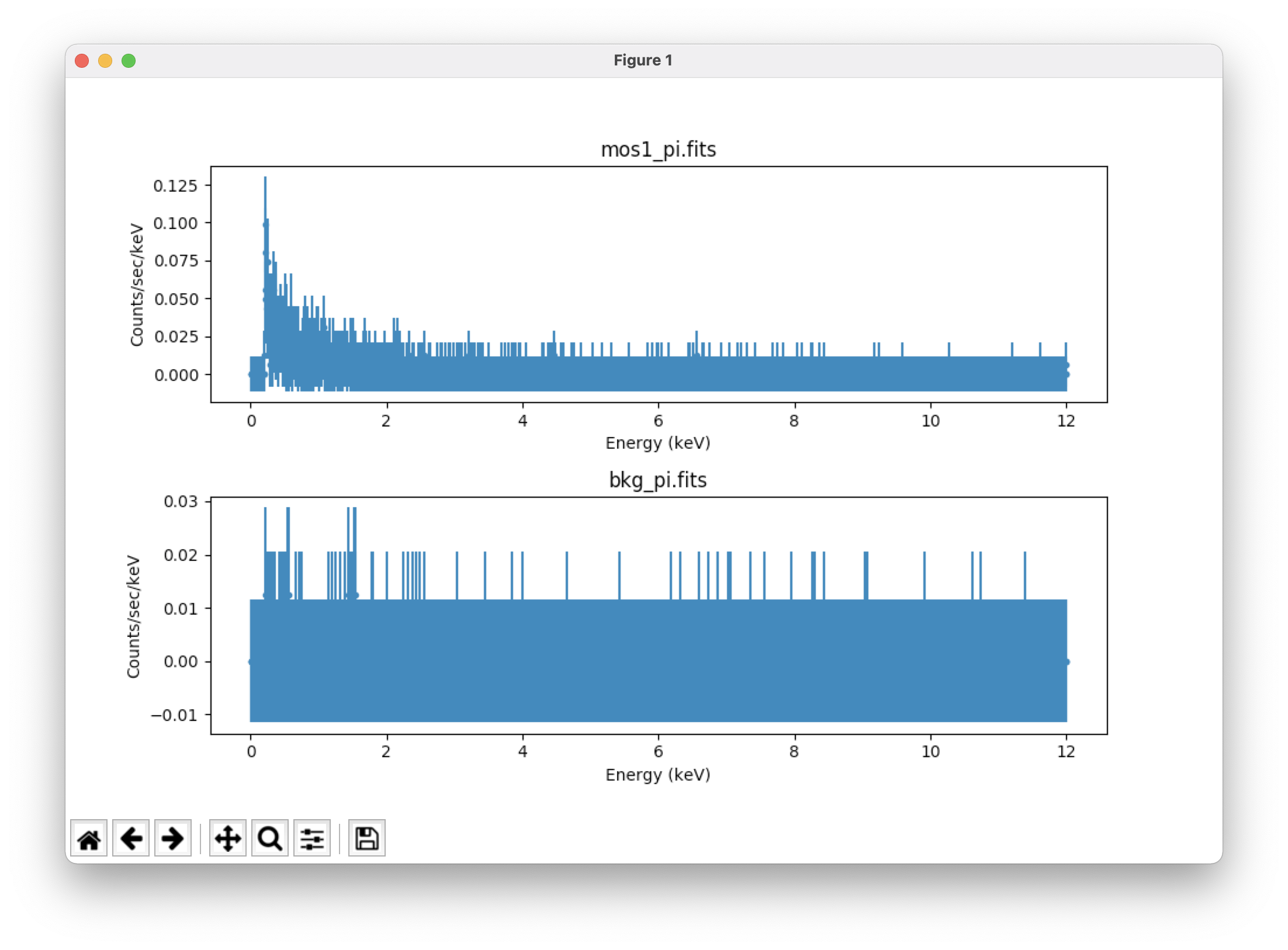
By default, Sherpa does not read in the uncertainties for the data points from the input file (though this can be changed). Rather, it calculates them depending on what statistic is chosen. The default statistic is Gehrel's χ2. These data have not yet been binned up such that that statistic applies, so the error bars in Figure 1 are not realistic.
We will first set the energy region that we are interested in, and then rebin so each bin has at least 20 counts, in excess of what is needed for Gehrel's χ2. This way, we don't have to worry about inadvertantly clipping the ends of the region, if the energy cut-off happens to fall in the middle of a bin.
ignore(":0.5,3:") # let's take only the data between 0.5-3 keV in both the source and background
ignore(":0.5,3:",bkg_id=1)
group_counts(20) # by default, both source and background are grouped
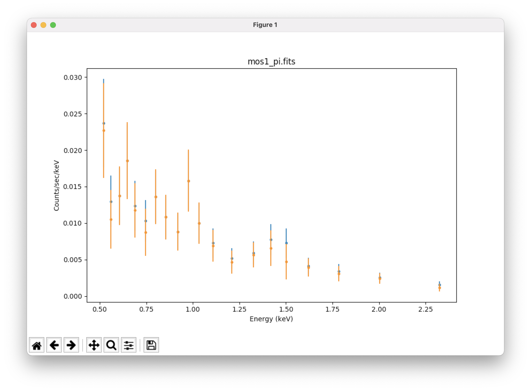
plot_data() # plot the data over that energy range
subtract() # subtract the background
plot_data(overplot=True) # overplot the subtracted spectrum on the unsubtracted one; see Figure 2 (top)
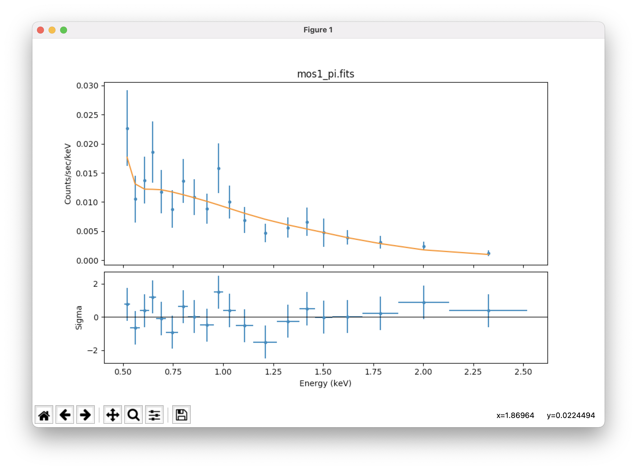
set_source(xspowerlaw.p1) # set a model for the source
fit()
calc_energy_flux(0.5,3) # get the source's energy flux from 0.5-3 keV in erg/cm2/s
plot_fit_delchi() # plot the fit and (data - model)/error; see Figure 2 (bottom)
|
Let's do this again, but this time, we'll fit the background. We'll assume it can be fit with a power law (which is not a great assumption; readers who are interested in learning more about how to fit the background are referred to the The Handbook of X-ray Astronomy). We will also change the fitting statistic and the optimization method. Since we will use cstat, there is no need to rebin the spectrum.
clean() # remove all data and fit information; this also resets the optimization and
# statistics settings to defaults if they were changed
load_pha("mos1_pi.fits")
ignore(":0.5,3:")
ignore(":0.5,3:",bkg_id=1)
set_stat("cstat") # Set the statistic from Levenberg-Marquardt to cstat
set_method("simplex") # simplex is the same as "neldermead" and samples a reasonably large
# amount of parameter space in a reasonably small amount of time
set_source(xspowerlaw.p1)
set_bkg_model(xspowerlaw.p2) # set a model for the background
fit() # automatically fits source and background simultaneously
conf() # estimate the uncertainties
set_stat("chi2gehrels") # cstat doesn't find errors on data points in fits, so we'll use Gehrel's χ2
# to estimate the errors in a plot
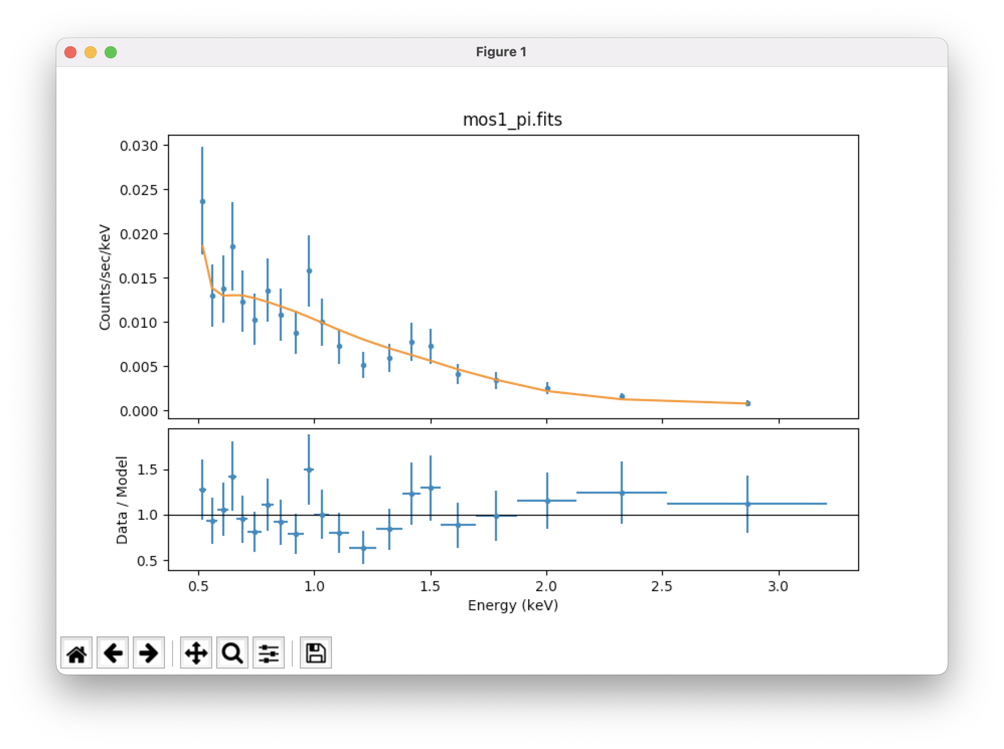
group_counts(20)
plot_fit_ratio() # plot the fit and the ratio of data/model
calc_energy_flux(0.5,3)
calc_energy_flux(0.5,3,bkg_id=1) # get the background's energy flux from 0.5-3 keV in erg/cm2/s
|
Let's do this one last time. Instead of using the source's response files, we'll use those of the background spectrum's. We will use "covar" instead of "conf" this time to find the errors. Covar is faster than conf; it freezes all other thawed parameters, while conf lets them float to new best-fit values. Conf samples the parameter space more widely than covar, but both are considered to be equally accurate if the models are relatively simple. If we were using models that were more complex, we would use conf.
   clean()
   load_pha("mos1_pi.fits")
   load_bkg_rmf("bkg_rmf.fits")   # read in the background's rmf file
   load_bkg_arf("bkg_arf.fits")   # read in the background's arf file
   ignore(":0.5,3:")
   ignore(":0.5,3:",bkg_id=1)
   plot("data", "bkg")
   set_stat("cstat")
   set_method("simplex")
   set_source(xspowerlaw.p1)
   set_bkg_model(xspowerlaw.p2)
   fit()
   covar()                        # quickly estimate the uncertainties
   exit()
More information about Sherpa, including models and commands and analysis threads can be found here.
If you have any questions concerning XMM-Newton send e-mail to xmmhelp@lists.nasa.gov