

Data Simulation and Analysis Threads
Fit an EPIC Spectrum with XSpec
For this example, we will first do a quick fit to see what we are dealing with, so we will rebin the spectrum, subtract the background, and fit the source. Then, we will do a simultaneous fit of the source and background, using each spectrum's associated response files.
The example data set is from the Lockman Hole (ObsID 0123700101) observation that we reprocessed. SAS typically doesn't play well with other software, so it is always recommended to keep it and your analysis software in different windows.
We will use two versions of the dataset: one that is rebinned, for plotting purposes and for fitting with the χ2 statistic, and the unbinned one, for fitting with cstat. (The binned spectrum could also be fit using cstat, but rebinning isn't necessary with cstat.) We can rebin the spectrum, and edit the headers so that XSpec will automatically load the auxilliary files, with the ftool "grppha".
   ftools
   grppha infile='mos1_pi.fits' outfile='mos1_pi_h_bin20.fits' chatter=0 \
      comm='group min 20 & chkey BACKFILE bkg_pi.fits & \
      chkey RESPFILE mos1_rmf.fits & chkey ANCRFILE mos1_arf.fits & exit'
Now we start it up and see what we have. When using the "ignore" command, be careful about using either integers or reals: integers indicate channel space, and reals indicate energy space.
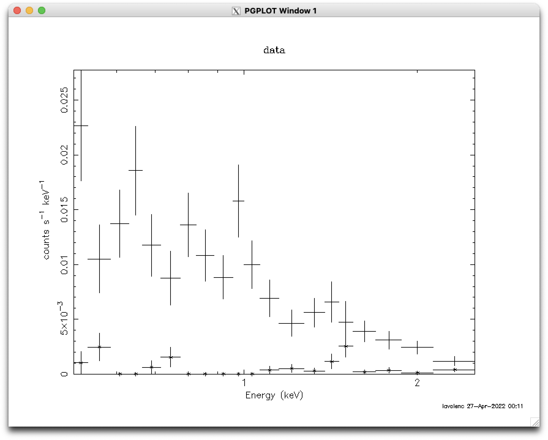
   xspec
   data mos1_pi_h_bin20.fits   # read in the source spectrum and any affiliated data from the header file
   cpd /xw                     # change the plotting device to xwindows
   setplot background          # when plotting a spectrum (or fit), also plot the background spectrum (or its fit)
   setplot energy              # plot in energy space
   ignore **-0.5,3.0-**        # let's take only the data between 0.5-3 keV
   plot data                   # plot the source and background on the same plot; see Figure 1
   show                        # see the specifics of the dataset and the XSpec settings
Now we will fit the spectrum. The background is automatically subtracted during the fit, and the default statistic, Gehrel's χ2, is appropriate. Let's set the initial parameter values to their defaults.
   model powerlaw             # define the model and initial parameter values; let's work with the
   <enter>                    # default values, so press "enter" until we return to the prompt
   <enter>
We can see that the initial χ2 value is quite large, ~ 5e11! This can be reduced this somewhat by having Xspec take a better guess at the normalization with the "renorm" command prior to fitting. Notice that when we call the "fit" command, Xspec gives us the uncertainties on the fitted parameters. However, these are not the formal errors, but rather general indicators of the fit! To find the formal errors, we must use the "error" command.
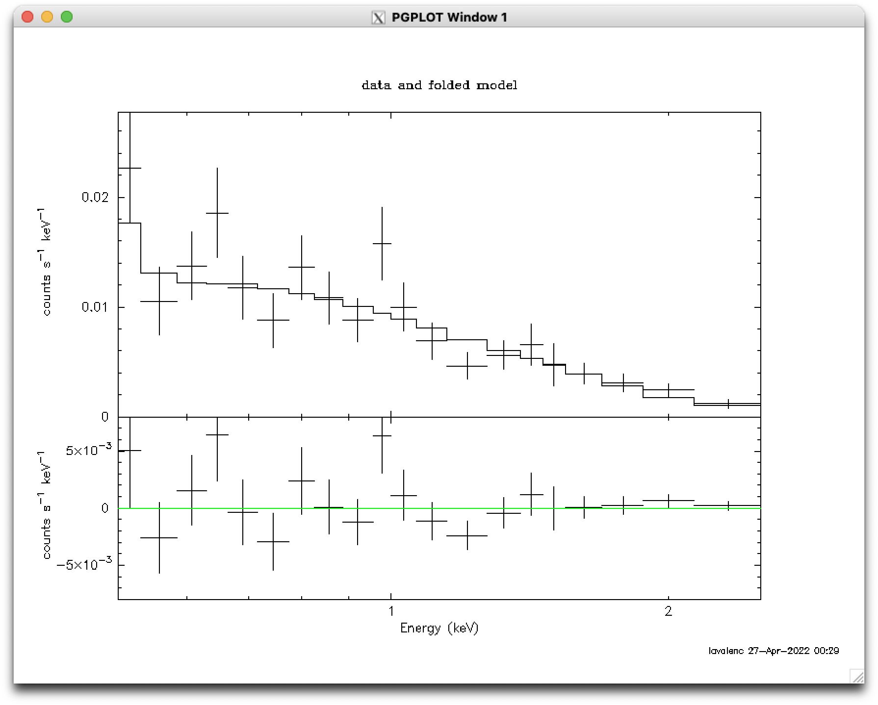
   renorm
   ignore bad                 # discard channels with poor quality
   fit
   error 1.0 1-2              # find the 1σ error bars on parameters 1 and 2
   flux 0.5 3.0               # get the source's energy flux from 0.5-3 keV in erg/cm2/s
   setplot nobackground       # turn off background plotting
   plot data resid            # plot the fit and residual
In the plot of the residual, the range on the y axis needs to be adjusted. We can do this with "iplot", though we should keep in mind that this will be plotted over the next time we plot something in Xspec.
   iplot
   window 2                   # apply the following commands to the second (lower) window
   rescale y -8e-3 8e-3       # tweak the y range; see Figure 2
   quit                       # return to the Xspec command line
   quit                       # exit Xspec; it will ask for confirmation (say yes!)
Let's do this again, but this time, we'll fit the background and use unbinned data. As before, we'll edit the headers to read in the response files for each spectrum.
   grppha infile='mos1_pi.fits' outfile='mos1_pi_h.fits' chatter=0 \
      comm='chkey RESPFILE mos1_rmf.fits & chkey ANCRFILE mos1_arf.fits & \
      chkey BACKFILE none & exit'

   grppha infile='bkg_pi.fits' outfile='bkg_pi_h.fits' chatter=0 \
      comm='chkey RESPFILE bkg_rmf.fits & chkey ANCRFILE bkg_arf.fits & \
      chkey BACKFILE none & exit'
Since we're not using binned data, we will change the fitting statistic to cstat; for
the test statistic, we'll use Pearson's χ2, which is appropriate for the
Poissonian regime.
   xspec
   statistic cstat
   statistic test pchi
   data 1:1 mos1_pi_h.fits 2:2 bkg_pi_h.fits    # read in the source and background spectra,
                                                # and their response files
Now we have to tell Xspec that there will be a background model, which must be
multiplied by the source's response files for its contribution to the source region,
and by the background's response files for its contribution to the background region.
We do this with the "response" and "arf" commands below.
   response 2:1 mos1_rmf.fits 2:2 bkg_rmf.fits
   arf 2:1 mos1_arf.fits 2:2 bkg_arf.fits
   ignore 1: **-0.5 3.0-**       # use only 0.5-3 keV in both spectra
   ignore 2: **-0.5 3.0-**
   model 1:src powerlaw          # the source's model; let's use the default values where we can
   <enter>
   <enter>
   <enter>
   0 0                           # the source model does not contribute to the background, so set its
                                 # normalization in the background spectrum to 0 and freeze it
   model 2:bkg powerlaw          # the background's model; we will use the default values for all.
   <enter>
   <enter>
   <enter>
   <enter>
   show param                    # display the values of all parameters
   renorm
   fit                           # both spectra are automatically fit simultaneously
   error 1.0 bkg:1-2             # find the 1-σ uncertainty in the background's parameters...
   error 1.0 src:1-2             # ... and the source's parameters
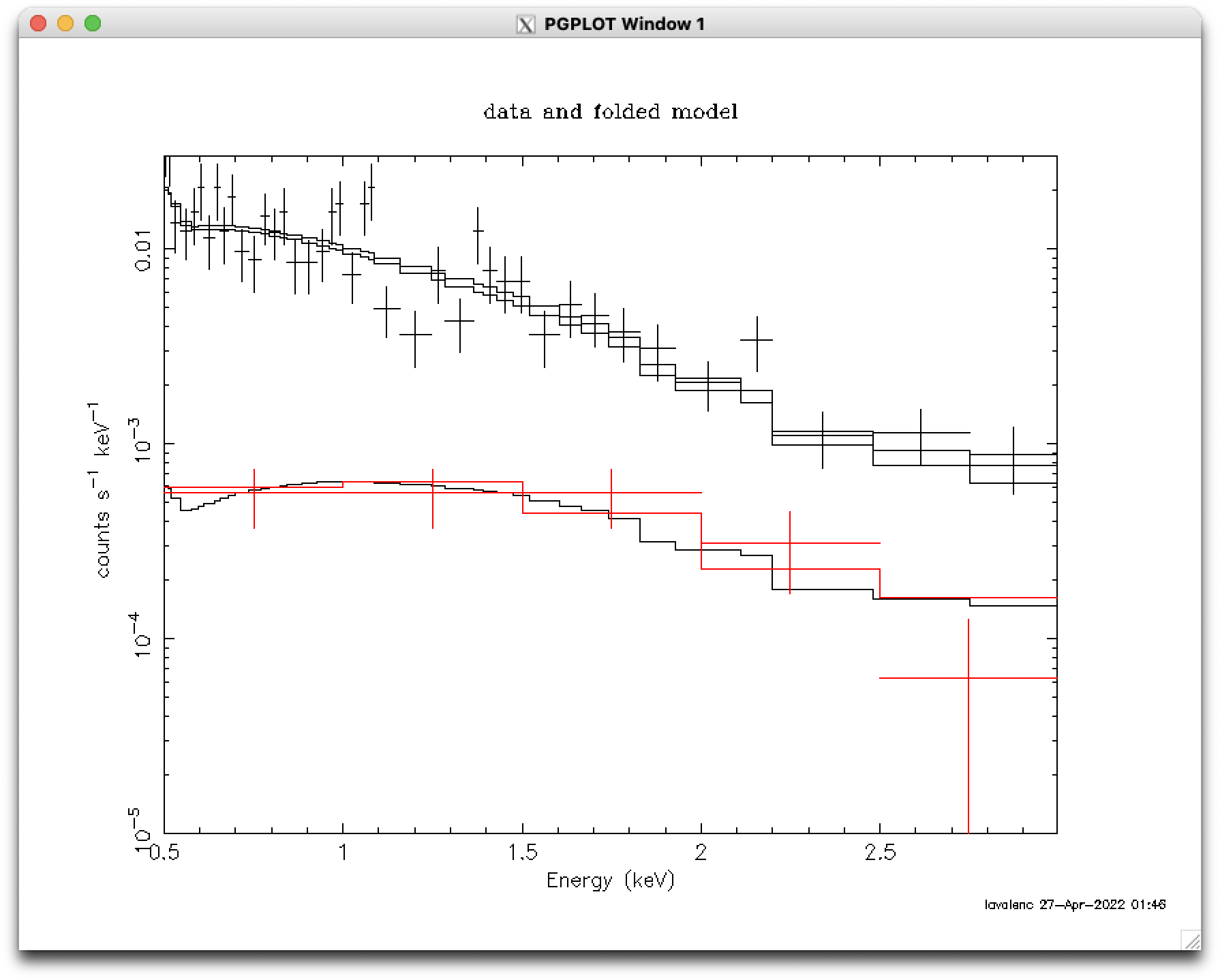
Now let's plot it. We rebin the data for clarity, keeping in mind that this does not affect the fit.
In the "setplot rebin" command below, we specify that adjacent bins are added until they have at least
a 3σ detection, but no more than 100 adjacent bins may be combined to meet this requirement.
   cpd /xw
   setplot energy
   setplot ylog on
   setplot xlog off
   setplot rebin 3,100,,
   plot
   iplot
   rescale y 1e-5 0.03            # see Figure 3
   quit                           # quit iplot
   quit                           # quit Xspec
More information about XSpec, including models and walk-throughs, can be found here.
If you have any questions concerning XMM-Newton send e-mail to xmmhelp@lists.nasa.gov