

Data Simulation and Analysis Threads
Simulate an EPIC, RGS, or OM Spectrum with Xspec
To simulate an EPIC spectrum, we will need an RMF and ARF that correspond to the mode and filter that we are interested in; for RGS, we need only an RMF; for OM, we need the RSP file for the filter we want (an RSP file is the product of the RMF and ARF, i.e., RSP = RMF × ARF).
An easy way to get the EPIC RMF and ARF files is to get the responses that are used for PIMMS and WebPIMMS simulations . Alternatively, we could download from the XSA archive an observation that was taken in the mode and filter we want, extract a spectrum and its associated RMF and ARF, and then use those response files to make a simulation. (While the mode and filter information is also in the HEASARC archive, observations are not easily searchable on these.) Note that the ARF is not time-dependent like the RMF is, so one from early in the mission should work well. However, ARFs are dependent on the filter, so be careful to select a dataset with the correct one. Or, if we prefer, we could download an observation in the mode and filter we want and then download a canned redistribution matrix with the corresponding epoch, mode, etc., and generate its corresponding ARF. Canned redistribution matrices for EPIC and RGS (and RSP files for OM) can be found through the SOC's calibration portal or the GOF ( PN, MOS, RGS, OM).
We will demonstrate how to simulate a point source, a source with background, and an OM source.
In this example, we assume that a source spectrum is known to be a power law with photon index=1.9, a Galactic absorption column of NH=5e21 cm-2, and an X-ray flux (0.2-12 keV) = 2.5e-12 erg s-1 cm-2. Let's say that we want to see what exposure time we need in order to measure the hydrogen column density to 2%. We need to initialize ftools and call Xspec.
   ftools
   xspec
   xsect vern                     # use the atomic cross sections of Verner et al. 1996
   abund wilm                     # use the elemental abundances of Wilms et al. 2000
   model (tbabs * powerlaw)       # define the model
When we define a model, Xspec will prompt us for parameter values.
   0.5                            # set NH to 0.5
   1.9                            # set photon index to 1.9
   1.0                            # the default normalization (= 1.0) is fine
   fakeit none
The "fakeit none" command will prompt us for a lot more information. At the last prompt, it will ask for three things: exposure time, correction norm, and background exposure time; just enter the exposure time.
   m1.rmf                         # our response file
   m1.arf                         # our ancillary file
   y                              # use counting statistics in making fake data?
   <enter>                        # optional fake name prefix
   mos1_sim_200ks.fits            # fake data file name
   2e5                            # enter the exposure time
Let's take a look at the flux this gives us in our chosen energy range. Be aware that in the "ignore" command below, our choice of integer or real values matters: if we enter integers, Xspec will assume we are referring to channels; if we enter reals, it will assume we are referring to energy (in keV).
   flux 0.2 12.0                  # find the flux in erg s-1 cm-2 from 0.2-12 keV; we
                                  # get 4.2637e-09
   ignore **-0.2 12.0-**          # only use 0.2-12.0 keV
   show all                       # show all information about the data and any model associated with
                                  # it; we can see that there are 4.88e+07 counts between 0.2-12 keV
When we use a normalization = 1, we get an energy flux in this passband of 4.2637e-09
erg s-1 cm-2. But we know that the flux should be 2.5e-12
erg s-1 cm-2. This means that we need to scale our normalization
accordingly:
( 2.5e-12 erg s-1 cm-2 / 4.2637e-09 erg s-1 cm-2) × 1.0 = 0.00058635
Parameter values can be changed (and tied together, and many other things) with "newpar".
   newpar 3 0.00058635            # set parameter 3 to 0.00058635
   fakeit none
   m1.rmf
   m1.arf
   y
   <enter>
   mos1_sim_200ks.fits
   y                              # Xspec will ask if it should overwrite the old file -- yes!
   2e5
What if we wanted to simulate a spectrum in RGS? The method is almost exactly the same, the only difference being that RGS does not have an ARF file. So to simulate the RGS1 first order spectrum, in the call to fakeit, we would simply enter None for the ARF:
   fakeit none
   R1o1.rmf
   None
   y
   <enter>
   r1o1_sim_200ks.fits
   y
   2e5
Returning our attention to the simulated MOS1 spectrum, it is a good idea to verify that we can recover the spectrum parameters. We can fit it using the same model that we used when making it, though we should first reset the initial values. We are not grouping the data and there is no background, so we will use cstat for the fit statistic and pchi for the test statistic. We can verify the new settings with the "show param" command.
   ignore **-0.2 12.0-**
   statistic cstat
   statistic test pchi
   newpar 1 1.0
   newpar 2 1.0
   newpar 3 1.0
   show param
Notice that with our new choice of initial value for the normalization, the C-statistic value is very large. We can reduce it by having Xspec take an educated guess at the norm with the command "renorm". (We should always do this when preparing to fit any spectrum, to increase our chances of getting a better fit faster.) When examining the output from "fit", we'll see that Xspec presents us with error estimates for each parameter. Be aware that these are given only as a general indicator of the errors, and are not the formal uncertainties! To find the correct uncertainties, we must use the "error" command.
   renorm
   fit
   error 1.0 1-3                  # get the 1-sigma error bars for all three parameters
We can see that the fit produced spectrum parameters in excellent agreement with their true values, and the percent error on NH is 2%, so this is a reasonable exposure time for our purposes.
Now we will rebin the data and plot the fit. Please note that rebinning is only for plotting purposes, and has no effect on the fit! This is done with the "setplot rebin" command, which lets us rebin to a certain chosen detection significance. As part of the command, we can also choose the maximum number of bins to combine in order to reach our desired detection significance, and how we want Xspec to calculate the uncertainty on the new bins. By default, this is set to addition in quadrature.
cpd /xw # call the XWindows plotting device
setplot energy # plot in terms of energy (keV)
setplot xlog on # log scale on the X axis
setplot ylog on # log scale on the Y axis
setplot rebin 5,1000,, # rebin to at least a 5 sigma detection level, or combine
# up to 1000 bins into a new bin
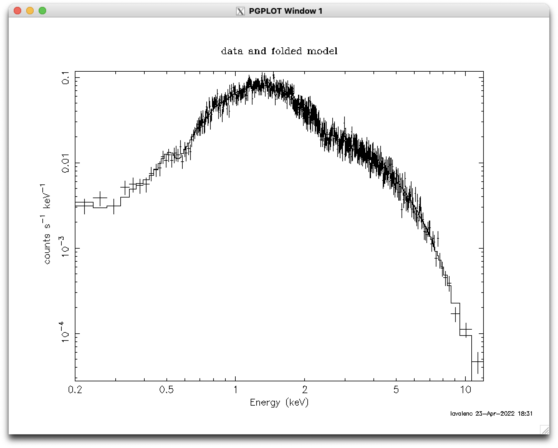
plot # see Figure 1 (top)
plot counts # plot the number of counts per bin; see Figure 1 (middle)
Let's tweak the minimum and maximum values on the Y axis and add a plot showing a comparison
of the fit to the data; while we're at it, we should also change the color of the fit line
to make it easier to see. To do this, we'll need to call "iplot" within xspec, which will put
us in the PLT environment and let us adjust various plot attributes. PLT uses vectors to
identify what is on the plot, with the data being '1' and the fit in '2'. Notice that the
changes made in iplot will be overwritten the next time we make a plot outside of iplot.
Notice also that changed colors will not be redrawn immediately but will be redrawn with
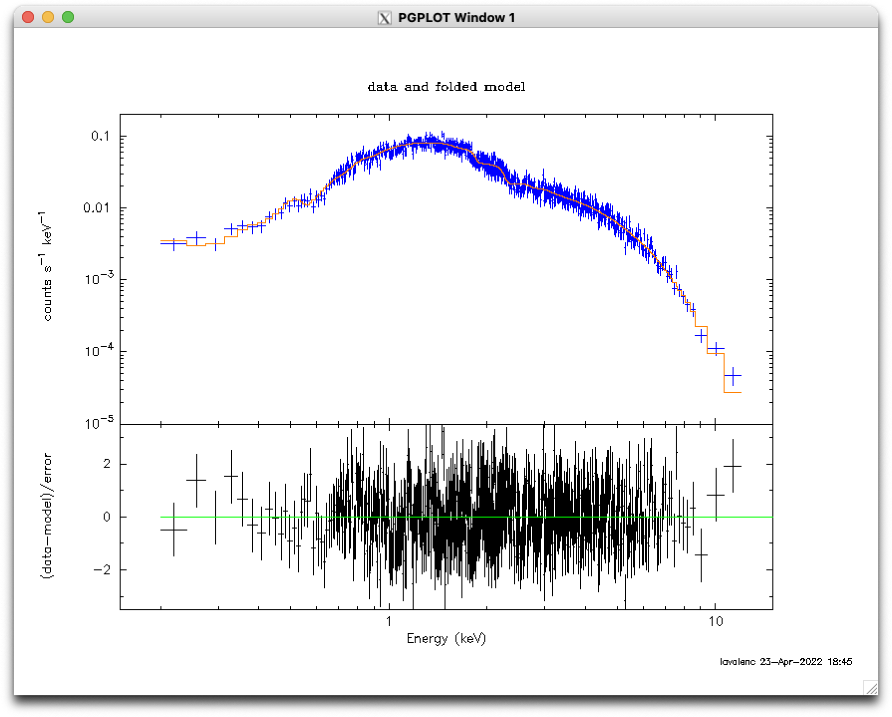
a "plot" or "rescale" command. The tweaked comparison image can be seen in Figure 1 (bottom).
   plot data delchi
   iplot
   co ?                 # list all the available colors
   window 1             # for the first window, apply the following commands
   co 4 on 1            # put color 4 (blue) on vector 1 (data)
   co 8 on 2            # put color 8 (orange) on vector 2 (fit)
   rescale y 1e-5 0.2   # set the Y axis range to 1e-5 to 0.2 count/s/keV
   window 2             # for the second window, apply the following commands
   rescale y -3.5 3.5   # set the Y axis range to -3.5 to 3.5
   window all           # for all windows, apply the following commands
   rescale x 0.15 15    # set the X axis range to 0.15-15 keV
   exit                 # return to the xspec prompt
|
|
A Source with a Background Component
We can also simulate a source with a background component. For convenience, we will use the same RMF and ARF as the source. Let's say that it is a standard AGN-dominated background, with photon index = 1.4 and an X-ray flux of about 1e-14 erg s-1 cm-2 in the bandpass. We must first simulate it on its own, to determine its normalization, and we will assume that the interstellar absorption is dominated by material between the source and us (i.e., there is negligible additional absorption in the AGN background).
   model (tbabs * powerlaw)
   0.5
   1.4
   1.0
   fakeit none
   m1.rmf
   m1.arf
   y
   <enter>
   mos1_sim_200ks_bkg.fits
   2e5
Using the method above, we see that for a flux of 1e-14 erg s-1 cm-2 between 0.2-12 keV, we need a normalization of 1.13812e-06.
   newpar 3 1.13812e-06  # set the third parameter to 1.13812e-06
   fakeit none
   m1.rmf
   m1.arf
   y
   <enter>                       # optional fake file prefix
   mos1_sim_200ks_bkg.fits
   y                             # overwrite the old file?
   2e5
We can exit out to clear the memory and load the faked source and background data and fit them. The names of the response files used to make them were automatically written into their headers, so they will load automatically.
   exit
   xspec
   xsect vern
   abund wilm
   statistic cstat
   statistic test pchi
   data 1:1 mos1_sim_200ks.fits 2:2 mos1_sim_200ks_bkg.fits
   ignore 1: **-0.2 12.0-**
   ignore 2: **-0.2 12.0-**
We will now define the model for the source, making sure to set the normalization for the fitting the background data to 0 and freezing it, since it doesn't contribute to the source model. For the other parameters, the default values are fine so just hit "enter".
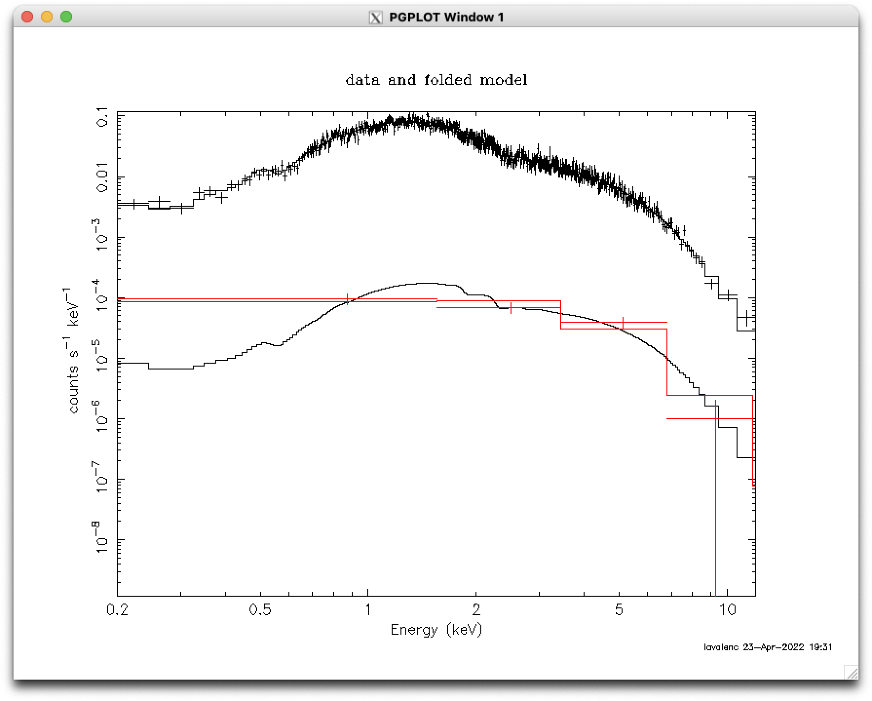
   model 1:src (tbabs * powerlaw)
   <enter>
   <enter>
   <enter>
   <enter>
   <enter>
   <enter>
   0 0
Now we have to tell Xspec that both these datasets have a second model which must be multiplied by the source's response matrix and ancilliary file for its contribution to the source region and the background's response matrix and ancilliary file for its contribution to the background region. In our example, these happen to be the same files. After this, we define the background model and use the default values for all parameters. We are treating absorbing column density as the same for both the background and source, so we will link the relevant parameters.
   response 2:1 m1.rmf 2:2 m1.rmf
   arf 2:1 m1.arf 2:2 m1.arf
   model 2:bkg (tbabs * powerlaw)
   <enter>
   <enter>
   <enter>
   <enter>
   <enter>
   <enter>
   newpar bkg:1 = src:1         # link the background's NH to the source's
   renorm
   show param
   fit
   error 1.0 bkg:2-3            # bkg:1 (NH) is linked to src:1, so Xspec won't find error on it
   error 1.0 src:1-3            # (but it will find it on the source's NH)
The plot of the rebinned data and fits to the source and background are in Figure 2.
OM data can be simulated in Xspec using the "fakeit" command just like X-ray data. As noted above, calling "fakeit none" will produce prompts for more information, including the response file and the ancillary file. There is only a .rsp file, so enter that for the response file and None for the ancillary file. Here, we will simulate an observation in the UVM2 filter with an exposure time of 1000 seconds. As before,
   ftools
   xspec
   model (powerlaw)
   fakeit none
   om_effarea_uvm2_v2.0.rsp              # The name of the response file
   None                                  # There is no ARF file.
   y                                     # Use counting statistics in creating fake data?
   <enter>                               # Input optional fake file prefix; we'll skip it.
   fake_uvm2.fits                        # Output file name
   1000                                  # Exposure time, correction norm, bkg exposure time \
                                         #    We will enter only the exposure time.
Xspec will complain that this is an ill-formed fit problem, but it will nonetheless
make the file, which will contain the "spectrum" (one data point!) of the number
of counts in the filter.
If you have any questions concerning XMM-Newton send e-mail to xmmhelp@lists.nasa.gov