Next: 7 Reference Guide
Up: User Examples
Previous: 6.1.1 Example 1: Processing
Back in Example 3 of Chapter 4, we performed an analysis of the Crab
spectrum, with particular emphasis on handling the pecularities of it being
a relatively hard source compared to many objects observed with OSSE.
Through the analysis, we obtained a `reasonable' spectrum but some might
have wondered why the spectrum seemed harder than expected, and had that
large break away from the power-law fit. In fact, there is indeed a
problem in that spectrum and it is one I demonstrate how to detect and fix
in this example.
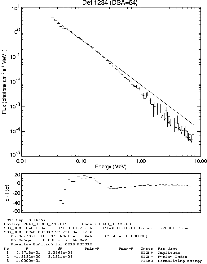
To see just how serious the problem is, let's take a closer look at the
spectrum generated for that example. Let's see how it looks with smaller
energy channels such as in Figure 6.3

Figure 6.3: A Spectrum of the Crab Nebula & pulsar from Viewing Period 221.
This was performed with the expanded response matrix and plotted with 100
logarithmically-spaced energy channels. The `kink' in the spectrum near 50
keV is not real! It is an instrument artifact.
The ``kink'' in the spectrum near 50 keV is not real. It is an instrument
artifact due to a change in the detector settings during the observation.
OSSE has a standard, normal gain (called ``x1 gain'') which provides energy
channels 6 keV wide below 1.5 MeV and 40 keV wide from 1.5 to 10 MeV.
Below 50 keV, electronic noise contributes to the spectra. In
twice-normal gain (``x2 gain'') the energy channels are 3 keV wide below
750 keV and 20 keV wide from 750 keV to 5 MeV and electronic noise doesn't
appear until below about 40 keV. However, below this energy, the OSSE
instrument itself has absorbed almost all the incident flux. Times-two
gain is very useful in observing soft sources.
IGORE performs most of its spectral manipulation operations in count-space
and photon energy doesn't come into the equation until FITIT
is performed. Prior to this, spectra are added channel by channel. The
problem arises because in normal gain, channel 20 may correspond to an
energy of 78 keV with a width of 6 keV. In x2 gain, channel 20 has an
energy of 37 keV and a width of 3 keV. The cause of the problem is that
you are adding two spectra, one translated and stretched with respect to
the other. The solution is to treat the two different gain settings
separately and only add them after they have been converted into photon-
space.
First we'll gather together the normal gain data and generate a spectrum.
Here is an IGORE program to do it:
Igore> sdr_load,'crabpulsar_221_gsm.sdb',sdr
Igore> gain=getfld('hdr.rgain',sdr)
Igore> tags=getfld('hdr.tagword',sdr)

Igore> exclude=tags(where(gain gt 1.5))  ; make an array of tags of x1 gain

Igore> ; regenerate response matrices with new range & exclude x2 gain
Igore> stat=ffit_prep(fileroot='CRABPULSAR_221x1',$
Igore>         sdbfile='CRABPULSAR_221_GSM.SDB',$
Igore>         Not_tags=exclude,$
Igore>         filesetup='NONE',$
Igore>         mtrx_nphot=600,$
Igore>         mtrx_prange=[0.02,20.0])

Igore> ; now reload it and fit it
Igore> sdr_load,'crabpulsar_221x1_tot.sdb',sdr
Igore> sdr$create,r_out,1
Igore> sdr_sum,sdr,r_out,/matrix              ; add them up
Igore> stat=fitit(fileroot='CRABPULSAR_221x1',$
Igore>         sdr=r_out,plot_nchan=100,$
Igore>         modelfile='PWRlaw.MOD')
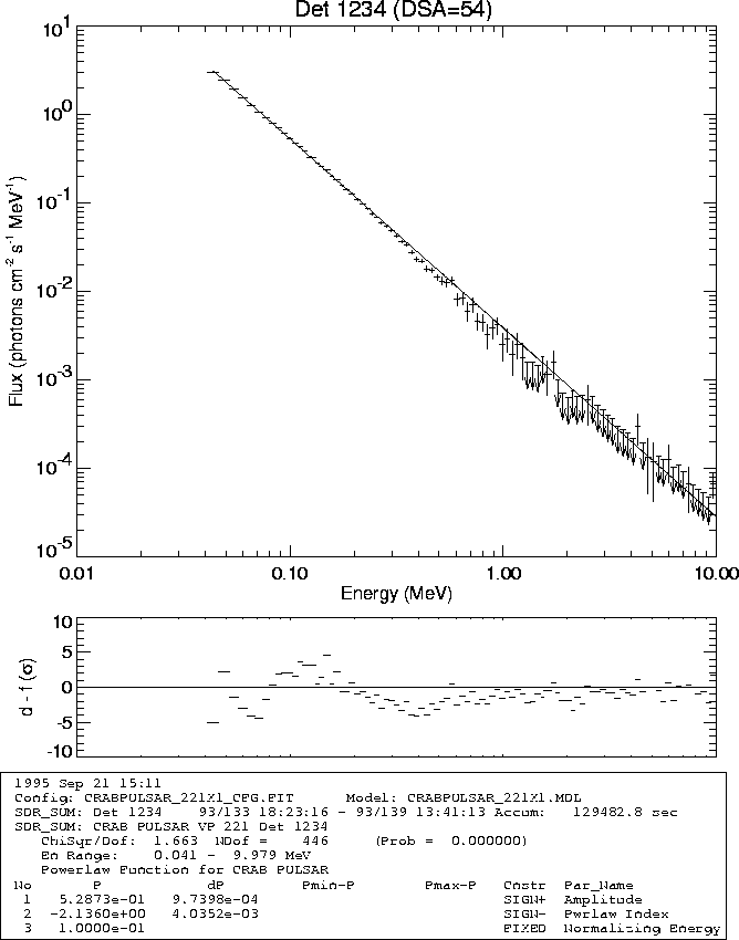
The results appear in Figure 6.4.

Figure 6.4: A Spectrum of the Crab Nebula & pulsar from Viewing Period 221
selecting normal gain data only. This was also performed with the expanded
response matrix and plotted with 100 logarithmically-spaced energy channels.
Note that the `kink' is gone.
Next we select out the x2 gain data and fit it. We'll use a different
method for extracting the data. It turns out that the EXCLUDE
keyword in FFIT_PREP can only handle up to 30 tags for
exclusion. For this next step, there are more than 30 SDRs which should be
excluded, so instead we create a new TOT.SDB file which contains only x2
gain data.
Igore> sdr_load,'crabpulsar_221_gsm.sdb',sdr,plus='crc,note'
Igore> gain=getfld('hdr.rgain',sdr)
Igore> index=where(gain gt 1.5) ; select x2 gain elements
Igore> write_specsdr,sdr(index),'Crab_tempx2_gsm.sdb'

Igore> ; regenerate response matrices with new range & only x2 gain
Igore> stat=ffit_prep(fileroot='CRABPULSAR_221x2',$
Igore>         sdbfile='CRAB_tempx2_GSM.SDB',$
Igore>         filesetup='NONE',$
Igore>         mtrx_nphot=600,$
Igore>         mtrx_prange=[0.02,20.0])

Igore> ; now combine the detectors
Igore> sdr_load,'crabpulsar_221x2_tot.sdb',sdr
Igore> sdr$create,r_out,1
Igore> sdr_sum,sdr,r_out,/matrix              ; add them up

Igore> ; fit the result
Igore> stat=fitit(fileroot='CRABPULSAR_221x2',$
Igore>         sdr=r_out,plot_nchan=100,$
Igore>         modelfile='PWRlaw.MOD')
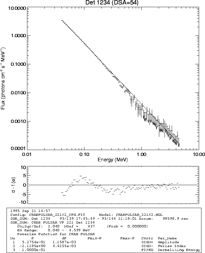
The results appear in Figure 6.5.

Figure 6.5: A Spectrum of the Crab Nebula & pulsar from Viewing Period 221
selecting twice-normal gain data only. This was also performed with the expanded
response matrix and plotted with 100 logarithmically-spaced energy channels.
Note that the `kink' is also gone here.
Next: 7 Reference Guide
Up: User Examples
Previous: 6.1.1 Example 1: Processing
