6. Data Analysis and Processing Software

In this chapter, we define and explain Suzaku software tasks that are used for the data processing at ISAS and GSFC and for the data analysis by Suzaku observers. The naming conventions of product files and directory structures can be found in more detail in the Interface Control Document (ICD)^6.1.

6.1 Overview

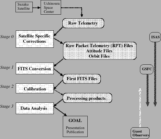
In figure 6.1, we provide an overview of the Suzaku data flow, which we divide into four stages: satellite specific calibration (Stage 0), production of the First FITS files (Stage 1), instrument specific calibration (Stage 2) and data analysis (Stage 3).

In general, software tools used in the earlier stages (Stage 0, 1) do not need to be portable since they run only at ISAS and/or GSFC, but they must be stable so that data need not be run through these stages repeatedly. On the other hand, software used in the later stages (Stage 2, 3) must be portable and flexible since they are distributed to Suzaku users for data analysis and for reprocessing when new calibration information becomes available. All distributable Suzaku software are built and distributed within the FTOOLS package (table 6.3 for a full list).

Figure 6.1: Overview of the Suzaku data flow.

6.2 Stage 0 - Satellite Specific Calibration

In this stage, the Suzaku team at ISAS collects the orbital information, processes satellite specific calibration, and converts satellite raw telemetry data and satellite specific information to the Raw Packet Telemetry (RPT) files, attitude FITS and orbital FITS files. The output RPS files are regularly copied to the database at GSFC as back-up (figures 2.1, 6.1 and 6.2).

6.2.1 Orbit Determination

JAXA/TKSC determines the Suzaku orbit and sends the data regularly to ISAS. The data are converted to FITS format, containing both the orbital elements as well as explicit satellite positions as a function of time during the relevant period.

6.2.2 Attitude Determination

The NEC/Toshiba space system develops the attitude determination software as for the GINGA and ASCA satellites. ISAS hires technicians who will work full-time on the attitude determination. The Suzaku attitude files have the same FITS format as the ASCA attitude files.

6.2.3 Raw Packet Telemetry Files

The Suzaku data are downlinked at USC, sent to ISAS and stored in the telemetry database, SIRIUS, of the ISAS data center,^6.2accessible through from UNIX workstations. SIRIUS embeds additional information into the original Suzaku telemetry when the Suzaku team accesses the data through the depacketer. The software astetimeset determines actual time corresponding to the satellite clock using the orbital information, and produces a timing correction (``tim'') file. The final products of the processing are Raw Packet Telemetry (RPT) FITS files, which have formats almost identical to the SIRIUS output, wrapped by the FITS header, as well as an orbit file, an attitude file, and a tim file. The maximum data size of one RPT is set at $\sim$2GB, and multiple RPT files can be produced if the data size exceeds the limit. An RPT file has three columns; TIME when a packet was created in Suzaku time (see section 4.1.1), the APID and the CCSDS packet.

6.3 Stage 1 - Production of the First FITS Files

The ISAS Suzaku team processes RPT files with the 1st Stage Software mk1stfits and produces the First FITS Files (FFF). The First FITS Files are composed of the event FITS files with the science data and HK files with the satellite and instrumental house keeping (HK) data. Since the electronic systems and coolers of the XRS are working and outputting the HK data through the Suzaku operation, the XRS HK data are generated regularly. Those files conform to the FITS standard defined by HEASARC.

The RPT files are used only to produce the First FITS Files at ISAS. Any other processes, such as the routine data reduction and the instrumental calibration, start with the First FITS Files. There are two exceptions of this rule.

• The hardware teams may test and debug the 1st Stage Software with the RPT files.
• The GSFC processing team may generate new version of the First FITS Files from the RPT files when the 1st Stage Software is revised.

ISAS shall routinely transfer to GSFC the RPT files, the 1st Stage Software and related files for back-up, the First FITS Files for the Stage 2 processing as necessary.

6.3.1 First Stage Software - mk1stfits

The 1st Stage Software is developed by the instrument teams, ISAS, and GSFC. It will not be distributed to the community, and therefore need not be portable. However, the 1st Stage Software shall be able to run both at ISAS and GSFC on some specific machines. The First Stage Software consists of the following components:

mkcom1stfits - binary executable for Common instruments (only create HK files)

mkxis1stfits - binary executable for XIS

mkhxd1stfits - binary executable for HXD

mkxrs1stfits - binary executable for XRS

xissubmode.pl - perl script for splitting the XIS data by the minor modes

mk1stfits - script to run the above software

The executables mk[com,xis,hxd,xrs]1stfits read a single RPT file, assign event time, reformat event data into standard FITS binary tables, convert raw digital HK readout to physical values and split a science FITS by major mode. The outputs are the First FITS files with the extension of ``fff", except for mkxis1stfits, which generates Temporary First FITS files (TFF) of the XIS data with the extension of ``tff". The perl script xissubmode.pl further splits the TFF files into different minor mode files, and output the First FITS files.

The major mode is defined as the modes with different event formats. For example, each of the 5x5, 3x3, 2x2 and timing modes corresponds to the XIS major mode, and each of the WELL main event data and WAM gamma-ray burst data does to the HXD major mode. Therefore, only from the event formats in the science data packet, the executable mk1stfits can split the data into the different major modes. The same major mode data in a single RPT file are put in one First FITS file even if they have time-gaps. For example, if the XIS major mode switches from the 5x5 mode to the 3x3 mode and then back to the 5x5 mode, the first and last 5x5 mode data are combined into one First FITS File. In other words, mk1stfits separates the input RPT file into different ``major'' observation modes, and generates a First FITS file for each major mode.

The minor mode is defined as the data sets that have different characteristics and cannot be analyzed together. For example, differences in exposure time of the Burst mode, parameters of the Window mode and numbers of vertical lines added in the Timing/Psum mode represent the minor modes. Since the science data have no change between the minor mode changes, xissubmode.pl refers to the HK information for the minor mode split. The on/off of the area discrimination is not regarded as the change of the minor modes, and is recorded in the EXPOSURES extension (section 6.4.2). Though the HXD well data have the minor mode in the clocking rate (CLKRATE), they are split at Stage 3-1, when making the cleaned event files (section 6.5.1). Moreover, CLKRATE is not supposed to change in 1 observing sequence, and therefore no split should be necessary in the Stage 3-1, either.

Table 6.1 lists the observation data types for the XIS and the HXD.

Mk1stfits should not lose any information in the RPT files (i.e. original telemetry) including low level instrument data, which are difficult to understand for general observers. It should generate columns of the physical quantities such as PI, GRADE and TIME, which are calculated in Stage 2, and fills them with a temporary value of ``$-$999.'' Likewise, the First FITS Files should contain all keywords necessary for analysis. The First FITS Files have a preliminary GTI table, which corresponds to the time intervals with the telemetry data, and does not depend on the instrumental status or observational conditions (see section 6.4.2 and 6.5.1). Mk1stfits internally calls functions in the standard FTOOLS package, so that the 1st stage processing should prohibit FTOOLS parameter files that it use to be overwritten by any other processes running in parallel.

6.3.2 Convention for naming First FITS Files

The First FITS Files consist of the science (event) files and the HK files. The root names of the First FITS Files are inherited from the RPT file name. For example, if a RPT file name is ae100037050_0.rpt, its First FITS File names always start with ae100037050_0.

6.3.2.1 Event Files (Science Files)

The RPT root name is followed by an instrument name, file number and a major mode name with underscores (``_'') between them. The instrument name is either xi0, xi1, xi2, xi3 or hxd and the major mode name is 5x5, 3x3, wam, or well, for example. The XIS major mode name is also followed by the onboard micro code number ranging from 0 to 255. The file number is 0 when a FFF is made from only one RPT or merged from multiple FFF files, otherwise 1 from the first RPT, 2 from the second FFF, and so on. The extension is ``.fff''.

Table 6.1: Observation data types

Instrument	Mode name
XIS	5x5, 5x5_burst
	3x3, 3x3_burst
	2x2, 2x2_burst
	timing_psum
	frame, frame_burst, frame_psum
	darkframe, darkframe_burst, darkframe_psum
	darkinit,darkinit_burst, darkinit_psum
	darkupdate, darkupdate_bst
HXD	wel, trn, bst_N
Note. -- N is numbered as the order of burst signals detected in an observing sequence.

Examples of the First FITS File names are shown below:

        ae100037050xi0_0_5x5n000.fff

ae100037020xi0_1_3x3n000.fff

ae100037050hxd_0_wam.fff

ae100037050hxd_0_wel.fff

ae100037050xrs_0_ff.evt

6.3.2.2 HK Files

Instrument names are the same as the event files. Suffix of the HK files is ``hk''. The HK identifiers, their meanings and examples are shown in table 6.2.

Table 6.2: The HK First FITS Files

Instrument	HK identifier	Meaning	Example
COM	none	common instrument HK	ae100037020.hk
	none	extended common HK	ae100037020.ehk
XRS	xrs	XRS HK	ae100037050xrs_0.hk
XIS	xi0,xi1,xi2,xi3	XIS HK for each sensor	ae100037050xi1_0.hk
HXD	hxd	HXD HK	ae100037050hxd_0.hk

Table 6.3: Suzaku FTOOLS list

Name	Order	Function
Attitude/Orbit
aemkehk		Generate attitude and orbit Extend HK (EHK) files
aemkreg		Generating region files of the XIS and HXD field of views
Common/Processing
makefilter		Generate a Filter file from HK and EHK files
Common/Analysis
aeattcor		Model the attitude wobbling due to the thermal distortion of the satellite body
aeaspect		Calculate the mean satellite Euler angle
aebarycen		Apply barycentric correction to Suzaku EVENT and HK files
aecoordcalc		Calculate coordinates
aetimecalc		Calculate mission time
suzakuversion		Report the version string for Suzaku package
aescreen		Carry out standard data screening of event files (under development)
mkphlist		Photon list generator for xissim
XIS
xisucode	XIS_S1	Fill the microcode information in the FITS header
xistime	XIS_S2	Fill the time column and the EXPOSURES column
xisgtigen	XIS_S3	Generate a FITS file with time interval without telemetry saturation
xiscoord	XIS_S4	Fill the sky coordinate columns
xisputpixelquality	XIS_S5	Fill the STATUS column
xispi	XIS_S6	Fill the XIS PHA, PI and GRADE columns
xisllefilter	XIS_T1	Read information of light leak from fff or sff and output to files
xisexpmapgen		calculate a detector mask image and an exposure map in the sky coordinates
xisputhkquality		Output an HK file without unimportant HK data (under development)
xisexposureinfo		Fill the EXPOSURES extension (under development)
xispsumtime (TBD)		Fill the time column for the timing mode data (under development)
xiscontamicalc		Calculate the XIS OBF contamination
xisrmfgen		Generate a detector response matrix
xisarfgen		Generate an auxiliary response matrix (under development)
xissim		XRT+XIS photon simulator
xissimarfgen		Generate an auxiliary response matrix from the XRT+XIS photon simulation
HXD-WPU
hxdtime	Well_S1	Fill the TIME column of the Well event file
hxdmkgainhist$^\dagger$	Well_S2	Generate a gain history FITS file
hxdmkgainhist_gso		Generate a HXD-well PMT gain history file
hxdmkgainhist_pin		Generate a HXD-well pin gain history file
hxdpi	Well_S3	Fill the PI column of the Well data using the gain history file
hxdgrade	Well_S4	Fill the GRADE column of the Well data
hxddtcor		Calculate the dead time correction for PHA files
hxdgtigen		Give the GTI to remove the telemetry saturation intervals
hxdarfgen		Generate a list of the ratio of efficiency at off-axis
hxdwamtime	Wam_S1	Fill the TIME column of the Wam event file
hxdmkwamgainhist$^\dagger$	Wam_S2	Generate a gain history FITS file of the WAM data
hxdwampi	Wam_S3	Fill the PI column of the WAM data using the gain history file
hxdwamgrade	Wam_S4	Fill the GRADE column of the WAM data
hxdmkwamlc		Make lightcurve(s) from the HXD WAM event file
hxdmkwamspec		Make spectra from the HXD WAM event file
hxdwambstid
hxdbsttime		Fill the TIME column of the gamma-ray burst event files
hxdmkbstlc		Make lightcurve(s) from the HXD Burst event file
hxdmkbstspec		Make spectra from the HXD Burst event file
hxdscltime	HK_S1	Assign time of the scaler HK data

The 2nd column shows the order to run tools in Stage 2 for Snumber and Stage 3 for Tnumber.
$^\dagger$: hxdmkgainhist and hxdmkwamgainhist read the SFF.

6.4 Stage 2 - Instrument Specific Calibration

The 2nd Stage Software, so called critical FTOOLS, apply the calibration information to the First FITS Files to generate the Second FITS Files (SFF). The major task is to populate columns of physical quantities, by referring to the calibration data. The critical FTOOLS are developed by the hardware teams in conjunction with the GSFC Suzaku GOF, and distributed to public as a part of the FTOOLS package (table 6.3). Both ISAS and GSFC run the pipe-line processing of this stage (section 6.6).

The 2nd Stage software may add new columns or keywords on the First FITS Files, but it should not remove any existing columns and keywords, so that the critical FTOOLS runs for the Calibrated FITS Files as well. This allows Suzaku users to re-calibrate the data from the Calibrated FITS files, without the First FITS files.

We explain the functions of the Critical FTOOLS by characteristics of tasks.

6.4.1 Stage 2-1 - Preprocess the Supplementary Data

• Determine the pointing direction

  The task aeattcor models the attitude wobbling due to the thermal distortion of the satellite body. Then, the task aeaspect calculates the average pointing direction from the corrected attitude file, and puts the result on the header keywords of the FFF products (event, hk, attitude and orbit). The result is later used as a reference point of the sky coordinate.

• Generate extended HK (EHK) files

  The task aemkehk extracts attitude and orbit information and generates ``Extended HK (EHK) Files'', which has the same format as the HK files, that is, a table of their physical value as a function of time.

• Produce a Filter file

  The analysis of the scientific data requires only a small part of the enormous HK information, such as detector temperature, count rates of the particle monitor, attitude and orbital information, magnetic cut-off rigidity, and intervals of the South Atlantic Anomaly (SAA) passages. The task makefilter extracts necessary HK items from the HK and EHK files into a filter file. Counting rates of the instruments and/or BGD monitors are also used for dead time correction (section 6.5.3).

6.4.2 Stage 2-2 - Refine the First FITS Event Files

• Correct event arrival time

  The task xisucode obtains information of XIS minor modes for the input 1st FITS files (FFFs) from a microcode list file in CALDB, and writes important parameters for calibration in header keywords of the input FFFs. Then, the task xistime corrects event arrival time in the normal, window and burst modes, which deviate $\mathrel{\hbox{\rlap{\hbox{\lower4pt\hbox{$\sim$}}}\hbox{$<$}}}$8 sec in the First FITS files. The timing mode data need further precise correction by referring to the RAWY coordinate with xispsumtime (TBD), which runs after the xiscoord populates the RAWXY columns.

  The task hxdtime calculates event arrival time from editing time of the event data packet.

• Update the GTI information

  The GTI extension in the First FITS File merely lists intervals with valid telemetry. It is updated in this stage with xistime for XIS and hxdtime for HXD, to list intervals when detectors are active and accumulating data from the Filter file. The xistime also lists exposure intervals of the burst mode. GTIs of the good observing condition such as low background and high elevation from the Earth rim are calculated in the Stage 3 (see section 6.5.1).

• Record the XIS exposure area

  The task xisexposureinfo (TBD) records onto the EXPOSURES extension the XIS exposure area, or more precisely, the area the data are taken and downlinked. The area discriminated by the onboard processor is excluded from the list. The list is written in the RAWXY coordinate by each CCD exposure. This information is used for making the exposure map, for example (section 6.5.3).

6.4.3 Stage 2-3 - Apply the Calibration Data

The event data are calibrated with the CALDB information to physical quantities or equivalent, which are filled in the corresponding columns.

• Calculate sky coordinate of XIS events

  The scientific analysis requires the photon arrival direction on the sky. The task xiscoord converts the detector coordinate of each event to the sky coordinate, with the reference to the XRT and XIS alignment calibration in CALDB and satellite attitude at the photon arrival time in the attitude file. The sky coordinate of each event and the reference R.A, Dec. coordinate are filled in the X/Y columns and the FITS header, respectively.

• Calculate PI from PHA

  The scientific analysis requires the photon energy of the detected events. The tasks xispi for XIS and hxdpi for HXD convert PHA (pulse heights) values measured with each detector to PI (pulse invariant) values, which scale to the physical energy of X-ray photons and therefore which are invariant between detector units. The result is filled in the PI column.

6.4.4 Stage 2-4 - Classify Events

• Classify events from the event pattern

  Both XIS and HXD events are classified by event grades, which are defined as the pattern of pulse heights (PH) of 3$\times$3 pixels for the XIS, and as the hit pattern of adjacent detector units and/or the coincidence with the anti-detector for the HXD. The grade information is used for particle background subtraction in Stage 3. The xispi and hxdgrade perform this task for the XIS and HXD data, respectively.

• Flag XIS events detected at certain pixels

  Events detected on certain pixels are likely to be non-X-ray events or X-rays from internal calibration source. The task xisputpixelquality flags those events in the STATUS column, some of which are removed in Stage 3. Pixels which are flagged are:

  Bad columns and flickering pixels: Some CCD pixels permanently or intermittently pour out or draw in charges by a defect of electronics on the CCD chips. Such pixels, called bad or flickering pixels, disguise their PH patterns as X-ray events. The XIS team also found from the on-ground calibration that the CCD pixels which are read after those bad or flickering pixels in the same CCD column are mostly insensitive to X-rays, and that the X-ray insensitive area appears as a column on the CCD chip.

  $^{55}$Fe calibration source: $^{55}$Fe calibration sources constantly illuminates two corners of each XIS detector. Background level of these areas is higher at around 5.9 and 6.4 keV.

  Segment boundary and rows with spaced charge injection and around: Rows with spaced charge injection (SCI) have charges artificially injected and do not have sensitivity to X-rays. Events detected at CCD segment boundaries and rows around the SCI rows do not have 5$\times$5 pixel information, and therefore the background level is higher than those of normal pixels.

The final products of the 2nd Stage are the Unscreened event files (the file extension of ``_uf.evt"). Those files are separated by instrumental modes and have all the necessary keywords and correct GTI extensions, which are required for extraction of the scientific data products. They still include intervals which is generally excluded for the scientific data analysis, such as high background and Earth occultation.

6.5 Stage 3 - Data Analysis

The Suzaku observers receive the Unscreened event files and supplementary files necessary for data analysis from ISAS or GSFC. For the scientific analysis, they need to be processed further: data screening to maximize data signal-to-noise ratio, event extraction from the aiming target and generation of the corresponding instrumental response. The instrument teams study the standard method of data screening and implement it in the pipe-line processing^6.3. The users may skip those processes by using the pipe-line products.

6.5.1 Stage 3-1 - Screen the Data

Data used for the scientific analysis should be contaminated as little as possible by background events. Through ground and on-board calibration, the instrument teams have studied data screening criteria that maximize the signal-to-noise ratio of the science data. The pipe-line processing applies this screening criteria to the Unscreened event files and outputs the Screened event files with the extension of ``_cl.evt". Here is the standard method of the data screening.

6.5.1.1 Split Data Sets by Minor Modes

The XIS can set on board different window, grade discriminator and event threshold, and the HXD can do on the clocking rate. The unfiltered files are not split for the different discriminators or threshold but this is taken into account in the stage 3 processing.

6.5.1.2 Generate Good Time Intervals using the Filter File

The users have to remove bad quality data taken in high particle background, inappropriate detector temperature, low elevation from the Earth rim, unstable satellite pointing, and so on. The generic task maketime calculates those intervals by referring to the HK parameters in the Filter file, and outputs Good Time Intervals (GTI), from which the users can extract events taken in the ``good interval".

6.5.1.3 Filter XIS Data Based on the Frame or Exposure

The Suzaku onboard processor processes XIS events by the unit of discrete ``frames'', which corresponds to one CCD exposure in the normal mode and to multiple exposures in the Window modes. The maximum data capacity of the telemetry is limited per frame, and any overflows are is automatically discarded. Data in such a frame, so called telemetry saturated frame, are useless without special treatments, and are removed from the dataset by the tool xisgtigen.

6.5.1.4 Filter Events

The instrument teams have studied detector signals through ground and on-board calibrations and found that certain types of events are more likely to be due to X-rays than others. Events satisfying such criteria are selected as X-ray events.

• Select XIS and HXD events from their event patterns

  X-ray or gamma ray events from the observing sources tend to fall in certain event grades, so that events with the other grades are discarded. The task fselect selects events with good grades (The XIS standard analysis picks up events with the grade 02346. The HXD grade selection is different between PIN and GSO and is complicated.)

• Remove flagged events

  The users may discard events flagged in the STATUS column (see section 6.4.4) using xselect. Events on the bad columns and flickering pixels simply increase the background level, and should be removed in any scientific analysis. While the $^{55}$Fe illumination produces strong background at $\sim$6 keV, it is almost negligible in the other bands. Therefore, events on the masking area can be useful for soft source analysis, for example. Those events are not removed in the Cleaned Event Files in the pipeline processing at ISAS and GSFC.

• Select HXD events in the Fast vs. Slow decay-time plane

  Fluorescent lights from both GSO and BGO scintillators in the WELL unit are detected with one PMT at the bottom. Since GSO has faster fluorescence decay time-scales than BGO, signals from GSO can be discriminated using the pulse shape. Practically, the analog electronics has Fast and Slow integration circuits with decaying time-scales of GSO and BGO, respectively. Pulses from GSO and BGO fall onto different regions on the two dimensional Fast vs. Slow circuit pulse height plane. With those information, the on-board PSD (Pulse Shape Discriminator) can discriminate and flag the GSO events. However, to check the on-board algorithm and to optimize the region in the Fast vs. Slow decay-time plane in on-ground data screening, the flookup task is available.^6.4.

• Select HXD PIN and/or GSO events

  An HXD Unscreened event file include all events which hit PIN, GSO, or both. The users can choose any sets of these events from the grade information using the task fselect.

6.5.1.5 Data Screening Script - aescreen [TBD]

The Suzaku data processing team will develop the Perl script aescreen [TBD], which carries out the sequence of the above data screening tasks automatically. The script will have options of the built-in tasks, which allow users to screen data with their own criteria. The script will run in the pipe-line processing with the standard criteria to produce the Screened event files (section 6.6). The script is also available for Suzaku users.

6.5.2 Stage 3-2 - Extract Scientific Products

The users finally extract events from the processed event files with their own scientific interest. They can produce images, light curves and spectra, which are time, energy or spatially-sliced in need. For such purposes, xselect, which calls the task extractor inside, is available.

The extraction conditions should be recorded on the produced FITS file header since they may be needed by downstream software, for example by the instrumental response generator. xselect and/or extractor may be modified for Suzaku specific requirements.

6.5.3 Stage 3-3 - Generate Analysis Specific Data Sets

The users may generate instrumental response matrices or correct the produced data (e.g. barycentric corrections and dead-time corrections). The results depend on instrumental conditions, analytical methods, and the coordinate of the observing target. The users may need to feed the FITS file and/or input instrumental or physical parameters, so that the software knows specific information of the data, such as observation date, detector temperature, event extraction region, sky coordinates of the target, and so on.

6.5.3.1 Generate Response Matrices for Spectral Analysis

To carry out spectral analysis, users need to know detector response to the incident X-rays.

From ground and onboard calibrations, the XRT and XIS teams have extracted information necessary to build two types of XIS spectral response matrices, RMF (Redistribution Matrix File) and ARF (Ancillary Response File), as for earlier X-ray satellites with CCD instruments, ASCA, XMM-Newton and Chandra. The two dimensional matrix, RMF, describes pulse heights of the CCD signal against the irradiated X-rays onto the CCD chip through the XIS optical blocking filter (OBF), whose flux is normalized at unity. The one dimensional matrix, ARF, describes the combination of telescope effective area and transparency of the XRT thermal shield and of contamination onto the OBF by X-ray energy.

The HXD team have generated on-axis detector response files. The flux from the source at off-axis is corrected by the auxiliary file, which describe the efficiency ratio relative to the on-axis source.

• Generate XIS RMFs

  High energy particles constantly bombard CCD chips and damage CCD pixels. The damaged pixels reduce charge transfer efficiency between CCD pixels, and a certain percentage of electron charges is lost before readout. This appears as an increase of noise so that the spectral resolution gradually deteriorates. Because the amount of charge loss during the charge transfer depends on both number of pixel transfers on a CCD chip and extent of damage of a pixel, which is proportional to the amount of irradiation of charged particles, detector responses are a function of the observation date and the detector coordinate. The RMF generator xisrmfgen feeds the extracted spectral FITS and the calibration files from CALDB, and outputs a RMF.

• Generate XIS ARF

  Observed photon counts depend on the shape of the source extracting region, the source position in the source region, off-axis angle of the source in the XRT field of view, and the shape of the X-ray source (ex. point or diffuse source). The ARF generator xisarfgen and xissimarfgen feed these information from the spectral file, response file and optional parameters, and output an ARF file.

• Generate HXD Response

  The HXD team have prepared on-axis response matrices, which include information of both the detector effective area and detector efficiency. Since it corresponds to the combination of RMF and ARF, the extension is ``rsp", as the convention of the response file combining RMF and ARF.

  The ARF file is not necessary for an on-axis point source. For an off-axis point source or diffuse source, the arf generator hxdarfgen calculates the observed flux ratio against the on-axis source and outputs an ARF file (section 7.4.4).

6.5.3.2 Generate XIS Exposure Maps and Vignetting Maps in Sky Coordinates

The exposure map describes exposure time of each pixel on the celestial (sky) coordinate system. The map is used when the users measure count rates of sources on an image or make a mosaic image from multiple images, along with the telescope vignetting map. The users first produce the exposure map of each pixel on the detector coordinate, from the exposure information in the EXPOSURES extension of the event file, bad column locations and the calibration-mask-area in the CALDB. From these information, the task makeexposuremap (TBD) converts the exposure map on the detector coordinate to the sky coordinate, by referring to the attitude file or the average Euler angle.

The vignetting map describes the telescope effective area and optionally instrumental efficiency. The telescope effective area on the detector coordinate in CALDB (section 7.4.2) has to be converted to the sky coordinate, to make a mosaic image.

6.5.3.3 Generate Background Files

The screened data still have a part of particle background and cosmic X-ray background, whose effect needs to be estimated from the off-source data. Generally, it is best to take the background from the same observation, to safeguard against possible background variation. Thanks to the imaging capability, the XIS data can easily provide a off-source region if an imaging size of an X-ray source is enough smaller than the XIS FOV. However, the HXD data without imaging information, or the XIS data of diffuse sources that cover the entire XIS FOV, need background from the other off-source observations. Suzaku observers may take an individual background data if they need a careful study of background contamination specific to the source, but the background data or model studied by the instrument team would be enough for most of the observations.

The instrument teams study the HXD and XIS background from the blank sky, the night Earth and day Earth data. For the XIS, non-X-ray background is accumulated from the night Earth data and the database is available from the trend archive. The users can extract background image or spectra from the event files using xselect. A task generates NXB spectra optimized for the observing and analyzing conditions such as exposure distribution against COR in an observation and event extracting regions (TBD). The database for this task will be stored in CALDB (TBD). For the HXD, the background level strongly increases after the SAA passage and internal background will gradually increase with time since high energy particles radio-activate PIN and GSO. The instrument team studies behavior of the background spectra in various conditions, generates database of events during earth occultation sorted with parameters sensitive to the background level, and reproduces background events for each observation from the database. The HXD team will prepare archives of background event files for each observation, or develop a tool to reproduce background events (hxdbackest: TBD).

6.5.3.4 Correct the HXD Dead Time

The HXD detector has non-negligible dead time in observations of X-ray sources at any flux level, because of the significant amount of particle background events at all times. The task hxddtcor derives correct exposure time, by counting pseudo events regularly generated by the onboard electronics.

6.5.3.5 Correct Event Arrival Time to the Solar System Barycenter

In the precise timing analysis such as the pulse search, event arrival time should be measured at the barycenteric frame of the solar system. The task aebarycen will convert event arrival time from the satellite frame to the barycentric frame.

6.5.4 Stage 3-4 - Derive Scientific Results

Suzaku users derive scientific results from these above products. For the analysis, the XANADU packages, XIMAGE (image), XRONOS (light curve) and XSPEC (spectrum) are available. If users need to re-extract scientific data or to change data screening criteria, they may return to Stage 3$-$2 or 3$-$1. Users may even go back to Stage 2 to recalibrate the data. However, there will never be the need to go back to Stage 1 (figure 6.1).

6.6 Pipeline Processing System

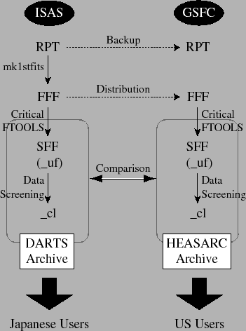
Most processing tasks in Stage 1-2 run automatically with a Perl script, whose system we call the pipeline processing (Figure 6.2). The script, developed at GSFC, runs at both GSFC and ISAS with the same versions of software and calibration files.^6.5Consistency of the products between GSFC and ISAS are regularly checked, using the checksum keywords in the FITS header. The pipeline processing mainly handles tasks in Stages 1, 2 and of the standard screening in Stage 3 (figure 6.1). Suzaku observers receive Unscreened event files and Screened event files and are expected to carry out the latter half of Stage 3.

Figure 6.2: Overview of the Suzaku data pipeline processing at ISAS and GSFC.

When software or calibration files are revised significantly, the pipeline reprocesses all earlier Suzaku data. The new products are shipped to Suzaku observers if the data are still proprietary, or they are updated in the Suzaku archives (chapter 9). Version names of the products are, for example, ver 0.1, ver 1.0, ver 2.0.