Each Suzaku proposal must include at a minimum the source coordinates, exposure time, instrument configuration and expected count rates, and any observing constraints within the four page limit. The review panels will base their decision primarily upon the justification of the proposed science to be done with the data. This chapter describes how to prepare a strong proposal, including the various software tools available to assist the proposer.
One of the first tasks in preparing a proposal is determining when and for how long a target can be observed as there is very little use to simulate a source that cannot be observed. This can be easily done with Viewing, a simple web-based interactive tool (see Appendix B) that can determine visibility for many different satellites. To use Viewing, simply enter the target name or coordinates, and select the satellite. Viewing will return all the available dates when that target is observable.
Another initial check to be performed before starting sophisticated
simulations is to ensure that the target has not yet been extensively
observed by Suzaku, e.g., using Browse. Users should also check
the observations log located at
http://heasarc.gsfc.nasa.gov/docs/suzaku/docs/suzaku/aehp_time_miss.html
as some of the targets (category C) may have been accepted but not
observed.
While it is conceivable that one would wish to study a previously unknown X-ray source with Suzaku, a more likely scenario would involve a spectroscopic study of an object with known X-ray flux. A viable proposal should state the scientific objective of the observation and show that Suzaku can achieve this objective. Observations that require one or more of Suzaku's unique capabilities would be especially strong candidates.
Every Suzaku proposal must have an estimate of the expected source count rates from the proposed target for all detectors. This rate is used both by the reviewers to evaluate the viability of the proposal and the operations team to evaluate any safety concerns. The simplest tool to use in estimating the expected XIS or HXD count rate is PIMMS. This tool is freely available as a stand-alone tool or on the web as WebPIMMS (see Appendix B). The next level of detail is provided via simulations using XSPEC, and such simulations should provide significant insight into the expected spectrum obtained from a proposed observation. A brief guide to XSPEC simulations is given in section 5.4. In many cases, this should be sufficient for a point source. There are also tools available to simulate imaging data, which may be useful for an extended source or a particularly bright source. In particular, the most powerful tool is xissim, which can use a FITS format image with an assumed spectral shape of the source to estimate the distribution of events in all elements of the XIS detectors.
PIMMS is an interactive, menu-driven program, which has an
extensive HELP facility. It is also available as the web-based tool
WebPIMMS. In either case, users specify the flux and spectral
model with its parameters, and PIMMS/WebPIMMS returns the
predicted count rate. PIMMS/WebPIMMS can be used for a variety
of other instruments, so if, for instance, the count rate and spectrum
of a given source observed with the ROSAT PSPC is known, PIMMS/WebPIMMS can estimate the expected count rates for Suzaku's
instruments. The limitations of the input source must be considered
carefully. For example, ROSAT had no significant response to
X-rays above ![]() keV, and so is not useful when estimating the
HXD GSO count rate.
keV, and so is not useful when estimating the
HXD GSO count rate.
Perhaps the easiest tool for simulating X-ray spectra is the XSPEC program (a part of the XANADU software package), which is designed to run on a variety of computer platforms and operating systems and is freely distributed on the NASA GSFC HEASARC web-site (see Appendix B). The simulation of an XIS observation requires the current instrument redistribution matrix (the so-called RMF file) and the energy-dependent effective area of the instrument (the so-called ARF file), while the simulation of an HXD observation requires the current instrument response (the so-called RSP file). These files are available on the Web or via anonymous FTP (see Appendix B).
The procedure for simulations is relatively simple: if the XSPEC program is installed, one should start XSPEC, making sure that the proper RMF, ARF, and RSP files are accessible. Within XSPEC, one should specify the spectral model, such as hot thermal plasma or the like (via the model command). Specifying the model will drive XSPEC to query for the model parameters (such as the temperature and abundances for an APEC collisional plasma model), as well as its normalization. The key command to create a simulated spectrum is the fakeit command, which will query for the RMF and ARF files, when simulating XIS, or for an RSP file, in the HXD case. The fakeit command will also request the data filename and the length of the observation to be simulated. One can then use the resulting spectrum within XSPEC to determine the sensitivity of the simulated data file to changes in the model parameters. Users should adjust the normalization of their input models to reflect the actual count rate or flux (absorbed or unabsorbed) of their source.
Some of the features of XSPEC are also available as a web-based tool on the HEASARC web-site (see Appendix B). WebSPEC calls XSPEC behind the scenes, so the description above applies here as well.
After selecting the instrument, WebSPEC allows the user to choose the spectral model, such as an absorbed collisional plasma or a power-law spectrum with an absorption component. The next page will then query for the model parameters (such as the temperature and abundances for an APEC collisional plasma model), as well as its normalization. In addition, it queries for the simulation parameters, i.e., the exposure, upper and lower energies, and the number of bins to use in the spectral plot. WebSPEC will then create a simulated spectrum after clicking the ``Show me the Spectrum'' button, using the fakeit command. This folds the specified model through the instrument response and effective area, calculating the observed count rate and fluxes as well. WebSPEC will then allow one to download the postscript file of the spectrum, change the model parameters, or re-plot the data.
In order to show how to estimate the proper exposure, we include some simple examples of XIS and HXD observations that illustrate the process.
The Local Hot Bubble is the proposed origin for at least some of the 1/4keV emission seen in the ROSAT All-Sky Survey at all latitudes. Although Suzaku has some sensitivity at 1/4keV, a more profitable approach to finding this emission is to detect the OVII emission that should accompany it. In this case we need to calculate the expected count rate from the OVII and compare it to the expected background.
We first need the expected flux, based on published papers or the PI's
model. In this case, we expect the surface brightness to be
0.34ph/cm![]() /s/sr, based on a number of papers. Since the XIS field
of view is
/s/sr, based on a number of papers. Since the XIS field
of view is ![]() , this value corresponds to a total surface
brightness in one XIS of
, this value corresponds to a total surface
brightness in one XIS of
![]() ph/cm
ph/cm![]() /s. The next
question is the effective area of the XIS instruments at the line
energy. OVII is in fact a complex of lines, centered around
0.57keV. Examining the effective area plots for the XIS in
Chapter 3, we see that the effective area at 0.57 keV
in the BI CCD is
/s. The next
question is the effective area of the XIS instruments at the line
energy. OVII is in fact a complex of lines, centered around
0.57keV. Examining the effective area plots for the XIS in
Chapter 3, we see that the effective area at 0.57 keV
in the BI CCD is ![]() cm
cm![]() ; for the FI CCDs it is
; for the FI CCDs it is ![]() cm
cm![]() . The curves shown on Fig. 3.3 do not include
the contamination effect. The computation below is only given as an
example. Please note that the more current effective area curves for
the FI and BI CCDs can also be found by loading their responses into
XSPEC and using the plot efficiency
command. Warning: The XIS RMF response matrices are not
normalized, and thus must be combined with the ARF files to determine
the total effective area. With the expected flux and the effective
area, we can now determine the expected count rate in the BI and FI
CCDs to be 1.3 and 0.87counts/ks. This is obviously a extremely low
count rate and so the expected background is very important. The
resolution of the XIS is quite good, as shown in
Chapter 7, at 0.57keV a bin of width 60eV will
contain most of the emission. The XIS background rate (see
section 7.3.4 at this energy is only 0.05counts/s/keV in both
the FI and BI detectors, so we can expect a background of
3counts/ks. In both the FI and BI detectors the line will be below
the background, but this does not intrinsically hinder detection. As
will be seen below, in the HXD this is the norm rather than the
exception. One aid for this observation is that the OVII line is
relatively isolated in this energy range, with the exception of the
nearby OVIII line. Assume we wish to detect the OVII
feature with
. The curves shown on Fig. 3.3 do not include
the contamination effect. The computation below is only given as an
example. Please note that the more current effective area curves for
the FI and BI CCDs can also be found by loading their responses into
XSPEC and using the plot efficiency
command. Warning: The XIS RMF response matrices are not
normalized, and thus must be combined with the ARF files to determine
the total effective area. With the expected flux and the effective
area, we can now determine the expected count rate in the BI and FI
CCDs to be 1.3 and 0.87counts/ks. This is obviously a extremely low
count rate and so the expected background is very important. The
resolution of the XIS is quite good, as shown in
Chapter 7, at 0.57keV a bin of width 60eV will
contain most of the emission. The XIS background rate (see
section 7.3.4 at this energy is only 0.05counts/s/keV in both
the FI and BI detectors, so we can expect a background of
3counts/ks. In both the FI and BI detectors the line will be below
the background, but this does not intrinsically hinder detection. As
will be seen below, in the HXD this is the norm rather than the
exception. One aid for this observation is that the OVII line is
relatively isolated in this energy range, with the exception of the
nearby OVIII line. Assume we wish to detect the OVII
feature with ![]() significance. The total count rate in the
XIS-S1 (the BI CCD) in our energy band will be 4.3counts/ks, with
3counts/ks of background. In an Nks observation, we will measure
the signal to be
significance. The total count rate in the
XIS-S1 (the BI CCD) in our energy band will be 4.3counts/ks, with
3counts/ks of background. In an Nks observation, we will measure
the signal to be
![]() . To achieve a
. To achieve a
![]() result, then, we need
result, then, we need
![]() , or
, or ![]() ks.
ks.
Another common observation will be to search for faint hard X-ray tails from sources such as X-ray binaries. We describe here how to simulate such an observation, including the all-important HXD background systematics, which will dominate all such observations.
The first step is to download the latest versions of the background
template files and the response files from the web-site listed in
Appendix B. The HXD web-site will also describe the
current best value for the systematic error in background estimation.
For this AO, proposers should carefully read Chapter 8
and evaluate the systematic errors for the PIN and the GSO backgrounds
in the energy band of interest, and at the exposure level chosen. For
example, for a 100ks exposure, the value for the PIN in the
15-40keV band and the GSO in the 50-100keV band can be
estimated to be ![]() 3% and
3% and ![]() 1.5%, respectively. Since the
energy bands are important in this case, the associated errors should
first be estimated and then used in the procedure described below. In
addition, the proposer should also check if contaminating sources
exist in the FOV of the HXD, using existing hard X-ray source catalogs
from satellites such as RXTE-ASM, INTEGRAL, and
Swift, before beginning this process.
1.5%, respectively. Since the
energy bands are important in this case, the associated errors should
first be estimated and then used in the procedure described below. In
addition, the proposer should also check if contaminating sources
exist in the FOV of the HXD, using existing hard X-ray source catalogs
from satellites such as RXTE-ASM, INTEGRAL, and
Swift, before beginning this process.
We set up XSPEC for simulating by reading the background template files as both data and background along with the response files:
XSPEC12>data ae_hxd_pinbkg_20101012.pha ae_hxd_gsobkg_20101012.pha

2 spectra  in use

Spectral Data File: ae_hxd_pinbkg_20101012.pha  Spectrum 1
Net count rate (cts/s) for Spectrum:1  4.735e-01 +/- 3.973e-04
 Assigned to Data Group 1 and Plot Group 1
  Noticed Channels:  1-256
  Telescope: SUZAKU Instrument: HXD  Channel Type: PI_PIN
  Exposure Time: 3e+06 sec
 Using fit statistic: chi
 No response loaded.

Spectral Data File: ae_hxd_gsobkg_20101012.pha  Spectrum 2
Net count rate (cts/s) for Spectrum:2  4.397e+01 +/- 3.829e-03
 Assigned to Data Group 1 and Plot Group 2
  Noticed Channels:  1-512
  Telescope: SUZAKU Instrument: HXD  Channel Type: PI_SLOW
  Exposure Time: 3e+06 sec
 Using fit statistic: chi
 No response loaded.

***Warning!  One or more spectra are missing responses,
               and are not suitable for fit.
XSPEC12>back ae_hxd_pinbkg_20101012.pha ae_hxd_gsobkg_20101012.pha
Net count rate (cts/s) for Spectrum:1  0.000e+00 +/- 5.619e-04 (0.0 % total)
Net count rate (cts/s) for Spectrum:2  0.000e+00 +/- 5.414e-03 (0.0 % total)
***Warning!  One or more spectra are missing responses,
               and are not suitable for fit.
XSPEC12>resp ae_hxd_pinxinome9_20100731.rsp ae_hxd_gsoxinom_20100524.rsp
Response successfully loaded.
Response successfully loaded.
We first create background spectra with the correct statistics, by
simulating an observation with no source flux using the fakeit
command. In the case of the PIN the simulated background exposure is
a factor 10 higher than the exposure of the source observation to be
simulated (here 10![]() s), following the prescription for PIN data
analysis. In the case of the GSO the simulated background exposure is
equal to the exposure of the source observation (here 10
s), following the prescription for PIN data
analysis. In the case of the GSO the simulated background exposure is
equal to the exposure of the source observation (here 10![]() s).
s).
XSPEC12>model powerlaw

Input parameter value, delta, min, bot, top, and max values for ...
              1       0.01(      0.01)         -3         -2          9         10
1:powerlaw:PhoIndex>1
              1       0.01(      0.01)          0          0      1e+24      1e+24
2:powerlaw:norm>0

========================================================================
Model powerlaw<1> Source No.: 1   Active/On
Model Model Component  Parameter  Unit     Value
 par  comp
   1    1   powerlaw   PhoIndex            1.00000      +/-  0.0
   2    1   powerlaw   norm                0.0          +/-  0.0
________________________________________________________________________


 Chi-Squared =            0.0 using 768 PHA bins.
 Reduced chi-squared =            0.0 for    766 degrees of freedom
 Null hypothesis probability =   1.000000e+00

***Warning: Chi-square may not be valid due to bins with zero variance
            in spectrum number(s): 1 2

 Current data and model not fit yet.
XSPEC12>fakeit
 Use counting statistics in creating fake data? (y):
 Input optional fake file prefix:
 Fake data file name (ae_hxd_pinbkg_20101012.fak): pin_10mCrab_1Ms.bkg
 Exposure time, correction norm, bkg exposure time (3.00000e+06, 1.00000, 3.00000e+06):
                                                                          1000000
 Fake data file name (ae_hxd_gsobkg_20101012.fak): gso_10mCrab_100ks.bkg
 Exposure time, correction norm, bkg exposure time (3.00000e+06, 1.00000, 3.00000e+06):
                                                                          100000

No ARF will be applied to fake spectrum #1 source #1

No ARF will be applied to fake spectrum #2 source #1

2 spectra  in use


 Chi-Squared =         637.77 using 768 PHA bins.
 Reduced chi-squared =        0.83260 for    766 degrees of freedom
 Null hypothesis probability =   9.997317e-01

***Warning: Chi-square may not be valid due to bins with zero variance
            in spectrum number(s): 1 2

 Current data and model not fit yet.
Now we assume a spectrum for our source; here, we use a Crab-like
spectrum (Toor & Seward 1974 AJ, 79, 995) with a photon index of 2.1,
a hydrogen column density N![]() of 3
of 3![]() 10
10![]() cm
cm![]() , and 10mCrab flux. This can be set up in XSPEC via
the following commands (note that while the response files are still
present from the previous step, the simulated background files from
the previous step should be loaded as background files, and the data
files do not matter):
, and 10mCrab flux. This can be set up in XSPEC via
the following commands (note that while the response files are still
present from the previous step, the simulated background files from
the previous step should be loaded as background files, and the data
files do not matter):
XSPEC12>back pin_10mCrab_1Ms.bkg  gso_10mCrab_100ks.bkg
Net count rate (cts/s) for Spectrum:1  2.101e-17 +/- 9.723e-04 (0.0 % total)
Net count rate (cts/s) for Spectrum:2  -3.640e-15 +/- 2.965e-02 (-0.0 % total)

 Chi-Squared =          3e-26 using 768 PHA bins.
 Reduced chi-squared =          4e-29 for    766 degrees of freedom
 Null hypothesis probability =   1.000000e+00

***Warning: Chi-square may not be valid due to bins with zero variance
            in spectrum number(s): 1 2

 Current data and model not fit yet.
XSPEC12>model phabs*powerlaw

Input parameter value, delta, min, bot, top, and max values for ...
              1      0.001(      0.01)          0          0     100000      1e+06
1:phabs:nH>0.3
              1       0.01(      0.01)         -3         -2          9         10
2:powerlaw:PhoIndex>2.1
              1       0.01(      0.01)          0          0      1e+24      1e+24
3:powerlaw:norm>0.097

========================================================================
Model phabs<1>*powerlaw<2> Source No.: 1   Active/On
Model Model Component  Parameter  Unit     Value
 par  comp
   1    1   phabs      nH         10^22    0.300000     +/-  0.0
   2    2   powerlaw   PhoIndex            2.10000      +/-  0.0
   3    2   powerlaw   norm                9.70000E-02  +/-  0.0
________________________________________________________________________


 Chi-Squared =       184046.2 using 768 PHA bins.
 Reduced chi-squared =       240.5832 for    765 degrees of freedom
 Null hypothesis probability =   0.000000e+00

***Warning: Chi-square may not be valid due to bins with zero variance
            in spectrum number(s): 1 2

 Current data and model not fit yet.
Now we can create fake PIN and GSO data for the planned observation using the fakeit command. The result will be simulated spectral files which include the instrumental background, effective area, and resolution:
XSPEC12>fakeit
 Use counting statistics in creating fake data? (y):
 Input optional fake file prefix:
 Fake data file name (pin_10mCrab_1Ms.fak): pin_10mCrab_100ks.fak
 Exposure time, correction norm, bkg exposure time (1.00000e+06, 1.00000, 1.00000e+06):
                                                                                100000
 Fake data file name (gso_10mCrab_100ks.fak): gso_10mCrab_100ks.fak
 Exposure time, correction norm, bkg exposure time (100000., 1.00000, 100000.): 100000

No ARF will be applied to fake spectrum #1 source #1

No ARF will be applied to fake spectrum #2 source #1

2 spectra  in use


 Chi-Squared =         660.11 using 768 PHA bins.
 Reduced chi-squared =        0.86289 for    765 degrees of freedom
 Null hypothesis probability =   9.974261e-01

***Warning: Chi-square may not be valid due to bins with zero variance
            in spectrum number(s): 1 2

 Current data and model not fit yet.
At this point we have created simulated spectral files for an
observation of a 10mCrab XRB, pin_10mCrab_100ks.fak and gso_10mCrab_100ks.fak. In order to achieve the statistics of an
actual observations, these files have to be rebinned to the spectral
binning of the regularly created GSO background files. A grouping file
which can be used with the FTOOL grppha is available
from
http://heasarc.gsfc.nasa.gov/docs/suzaku/analysis/gsobgd64bins.dat:
grppha gso_10mCrab_100ks.fak gso_10mCrab_100ks_bin.fak

  -------------------------
  MANDATORY KEYWORDS/VALUES
  -------------------------
  --------------------------------------------------------------------
  --------------------------------------------------------------------
  EXTNAME   - SPECTRUM        Name of this BINTABLE
  TELESCOP  - SUZAKU          Mission/Satellite name
  INSTRUME  - HXD             Instrument/Detector
  FILTER    -                 Instrument filter in use
  EXPOSURE  - 1.00000E+05     Integration time (in secs) of PHA data
  AREASCAL  - 1.0000          Area scaling factor
  BACKSCAL  - 1.0000          Background scaling factor
  BACKFILE  - gso_10mCrab_100ks_bkg.fak
  CORRSCAL  - -1.0000         Correlation scaling factor
  CORRFILE  - NONE            Associated correlation file
  RESPFILE  - ae_hxd_gsoxinom_20100524.rsp
  ANCRFILE  - NONE            Associated ancillary response file
  POISSERR  - TRUE            Whether Poissonian errors apply
  CHANTYPE  - PI_SLOW         Whether channels have been corrected
  TLMIN1    - 0               First legal Detector channel
  DETCHANS  - 512             No. of legal detector channels
  NCHAN     - 512             No. of detector channels in dataset
  PHAVERSN  - 1.1.0           OGIP FITS version number
  STAT_ERR  - FALSE           Statistical Error
  SYS_ERR   - FALSE           Fractional Systematic Error
  QUALITY   - TRUE            Quality Flag
  GROUPING  - TRUE            Grouping Flag
  --------------------------------------------------------------------
  --------------------------------------------------------------------
GRPPHA[] group gsobgd64bins.dat
GRPPHA[] exit
 ... written the PHA data Extension
 ...... exiting, changes written to file : gso_10mCrab_100ks_bin.fak
 ** grppha 3.0.1 completed successfully
The same grouping has to be applied to the GSO background spectrum:
grppha gso_10mCrab_100ks.bkg gso_10mCrab_100ks_bin.bkg

  -------------------------
  MANDATORY KEYWORDS/VALUES
  -------------------------
  --------------------------------------------------------------------
  --------------------------------------------------------------------
  EXTNAME   - SPECTRUM        Name of this BINTABLE
  TELESCOP  - SUZAKU          Mission/Satellite name
  INSTRUME  - HXD             Instrument/Detector
  FILTER    -                 Instrument filter in use
  EXPOSURE  - 1.00000E+05     Integration time (in secs) of PHA data
  AREASCAL  - 1.0000          Area scaling factor
  BACKSCAL  - 1.0000          Background scaling factor
  BACKFILE  - gso_10mCrab_100ks_bkg.bkg
  CORRSCAL  - -1.0000         Correlation scaling factor
  CORRFILE  - NONE            Associated correlation file
  RESPFILE  - ae_hxd_gsoxinom_20100524.rsp
  ANCRFILE  - NONE            Associated ancillary response file
  POISSERR  - TRUE            Whether Poissonian errors apply
  CHANTYPE  - PI_SLOW         Whether channels have been corrected
  TLMIN1    - 0               First legal Detector channel
  DETCHANS  - 512             No. of legal detector channels
  NCHAN     - 512             No. of detector channels in dataset
  PHAVERSN  - 1.1.0           OGIP FITS version number
  STAT_ERR  - FALSE           Statistical Error
  SYS_ERR   - FALSE           Fractional Systematic Error
  QUALITY   - TRUE            Quality Flag
  GROUPING  - TRUE            Grouping Flag
  --------------------------------------------------------------------
  --------------------------------------------------------------------
GRPPHA[group gsobgd64bins.dat] group gsobgd64bins.dat
GRPPHA[exit] exit
 ... written the PHA data Extension
 ...... exiting, changes written to file : gso_10mCrab_100ks_bin.bkg
 ** grppha 3.0.1 completed successfully
In the next step we fit these datasets with the Crab-like model defined above. We will use three different background assumptions - low, medium, and high - which vary by as much as 3% and 1.5% for the PIN and the GSO, respectively. This takes into account the fact that the ``true'' background will likely vary within these limits. We load the simulated source files (rebinned for the GSO). The simulated background files from the first fakeit step (rebinned for the GSO) - pin_10mCrab_1Ms.bkg and gso_10mCrab_100ks_bin.bkg -, are loaded as background files as well as as correction files (``corfiles''), the latter allowing for an easy way to vary the total background within XSPEC.
XSPEC12>data pin_10mCrab_100ks.fak gso_10mCrab_100ks_bin.fak

Spectrum #: 1 replaced

Spectrum #: 2 replaced

2 spectra  in use

Spectral Data File: pin_10mCrab_100ks.fak  Spectrum 1
Net count rate (cts/s) for Spectrum:1  3.803e-01 +/- 3.000e-03 (44.6 % total)
 Assigned to Data Group 1 and Plot Group 1
  Noticed Channels:  1-256
  Telescope: SUZAKU Instrument: HXD  Channel Type: PI_PIN
  Exposure Time: 1e+05 sec
 Using fit statistic: chi
 Using Background File                pin_10mCrab_100ks_bkg.fak
  Background Exposure Time: 1e+06 sec
 Using Response (RMF) File            ae_hxd_pinxinome9_20100731.rsp for Source 1

Spectral Data File: gso_10mCrab_100ks_bin.fak  Spectrum 2
Net count rate (cts/s) for Spectrum:2  3.287e-01 +/- 2.970e-02 (0.7 % total)
 Assigned to Data Group 1 and Plot Group 2
  Noticed Channels:  1-64
  Telescope: SUZAKU Instrument: HXD  Channel Type: PI_SLOW
  Exposure Time: 1e+05 sec
 Using fit statistic: chi
 Using Background File                gso_10mCrab_100ks_bkg.fak
  Background Exposure Time: 1e+05 sec
 Using Response (RMF) File            ae_hxd_gsoxinom_20100524.rsp for Source 1


 Chi-Squared =         318.41 using 320 PHA bins.
 Reduced chi-squared =         1.0044 for    317 degrees of freedom
 Null hypothesis probability =   4.672303e-01

***Warning: Chi-square may not be valid due to bins with zero variance
            in spectrum number(s): 1 2

 Current data and model not fit yet.
XSPEC12>back pin_10mCrab_1Ms.bkg gso_10mCrab_100ks_bin.bkg
Net count rate (cts/s) for Spectrum:1  3.802e-01 +/- 3.000e-03 (44.6 % total)
Net count rate (cts/s) for Spectrum:2  3.261e-01 +/- 2.970e-02 (0.7 % total)

 Chi-Squared =         305.87 using 320 PHA bins.
 Reduced chi-squared =        0.96490 for    317 degrees of freedom
 Null hypothesis probability =   6.629651e-01

***Warning: Chi-square may not be valid due to bins with zero variance
            in spectrum number(s): 1 2

 Current data and model not fit yet.
XSPEC12>corfile pin_10mCrab_1Ms.bkg gso_10mCrab_100ks_bin.bkg
Net count rate (cts/s) for Spectrum:1  8.529e-01 +/- 3.000e-03 (64.3 % total)
 After correction of -4.727e-01 (using cornorm -1.000)
Net correction flux: 0.472657

Net count rate (cts/s) for Spectrum:2  4.427e+01 +/- 2.970e-02 (50.2 % total)
 After correction of -4.395e+01 (using cornorm -1.000)
Net correction flux: 43.9467


 Chi-Squared =   2.212409e+06 using 320 PHA bins.
 Reduced chi-squared =       6979.207 for    317 degrees of freedom
 Null hypothesis probability =   0.000000e+00

***Warning: Chi-square may not be valid due to bins with zero variance
            in spectrum number(s): 1 2

 Current data and model not fit yet.
XSPEC12>model phabs*powerlaw

Input parameter value, delta, min, bot, top, and max values for ...
              1      0.001(      0.01)          0          0     100000      1e+06
1:phabs:nH>0.3
              1       0.01(      0.01)         -3         -2          9         10
2:powerlaw:PhoIndex>2.1
              1       0.01(      0.01)          0          0      1e+24      1e+24
3:powerlaw:norm>0.097

========================================================================
Model phabs<1>*powerlaw<2> Source No.: 1   Active/On
Model Model Component  Parameter  Unit     Value
 par  comp
   1    1   phabs      nH         10^22    0.300000     +/-  0.0
   2    2   powerlaw   PhoIndex            2.10000      +/-  0.0
   3    2   powerlaw   norm                9.70000E-02  +/-  0.0
________________________________________________________________________


 Chi-Squared =   2.212409e+06 using 320 PHA bins.
 Reduced chi-squared =       6979.207 for    317 degrees of freedom
 Null hypothesis probability =   0.000000e+00

***Warning: Chi-square may not be valid due to bins with zero variance
            in spectrum number(s): 1 2

 Current data and model not fit yet.
We now experiment with different background levels, set by the value of ``cornorm''. A value of 0 gives the ``normal'' background, for example, 0.03 increases it by 3%, and -0.015 decreases it by 1.5%.
XSPEC12>cornorm 1-2 0.0
 Spectrum 1 correction norm set to 0
 Spectrum 2 correction norm set to 0

 Chi-Squared =         305.87 using 320 PHA bins.
 Reduced chi-squared =        0.96490 for    317 degrees of freedom
 Null hypothesis probability =   6.629651e-01

***Warning: Chi-square may not be valid due to bins with zero variance
            in spectrum number(s): 1 2

 Current data and model not fit yet.
XSPEC12>ignore 1:**-15. 70.-** 2:**-50. 600.-**
    40 channels (1-40) ignored in spectrum #     1
    70 channels (187-256) ignored in spectrum #     1
     1 channels (1) ignored in spectrum #     2
    12 channels (53-64) ignored in spectrum #     2

 Chi-Squared =         152.83 using 197 PHA bins.
 Reduced chi-squared =        0.78780 for    194 degrees of freedom
 Null hypothesis probability =   9.869519e-01
 Current data and model not fit yet.

XSPEC12>fit
                    Parameters
Chi-Squared  Lvl          1:nH    2:PhoIndex        3:norm
152.172       -3      0.986583       2.11789      0.101826
152.107       -4       5.56204       2.13807      0.109058
152.035       -5       6.34881       2.14176      0.110693
152.035       -6       6.39060       2.14198      0.110787
========================================
 Variances and Principal Axes
                 1        2        3
 8.9577E-07| -0.0002  -0.3165   0.9486
 3.3044E+02| -1.0000  -0.0035  -0.0014
 1.3350E-03| -0.0037   0.9486   0.3165
----------------------------------------

====================================
  Covariance Matrix
        1           2           3
   3.304e+02   1.145e+00   4.517e-01
   1.145e+00   5.168e-03   1.966e-03
   4.517e-01   1.966e-03   7.519e-04
------------------------------------

========================================================================
Model phabs<1>*powerlaw<2> Source No.: 1   Active/On
Model Model Component  Parameter  Unit     Value
 par  comp
   1    1   phabs      nH         10^22    6.39060      +/-  18.1780
   2    2   powerlaw   PhoIndex            2.14198      +/-  7.18907E-02
   3    2   powerlaw   norm                0.110787     +/-  2.74216E-02
________________________________________________________________________


 Chi-Squared =         152.04 using 197 PHA bins.
 Reduced chi-squared =        0.78369 for    194 degrees of freedom
 Null hypothesis probability =   9.884693e-01
XSPEC12>cpd /xs
XSPEC12>setplot energy
XSPEC12>plot ldata res
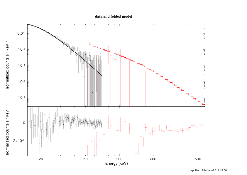
This result is shown in Fig. 5.1.
|
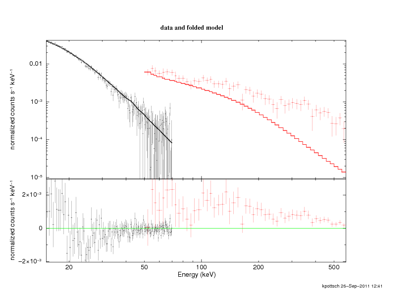
Now we check whether the same source signal would be detectable with a high background, i.e., a 3% and 1.5% higher background for the PIN and the GSO, respectively.
XSPEC12>cornorm 1 0.03 2 0.015
 Spectrum 1 correction norm set to 0.03
 Spectrum 2 correction norm set to 0.015

 Chi-Squared =         581.25 using 197 PHA bins.
 Reduced chi-squared =         2.9961 for    194 degrees of freedom
 Null hypothesis probability =   2.754551e-40
 Current data and model not fit yet.
XSPEC12>fit
                    Parameters
Chi-Squared  Lvl          1:nH    2:PhoIndex        3:norm
543.041       -2       2.65270       2.21924      0.127136
514.453       -2       4.29908       2.27391      0.153596
502.112       -2       15.5709       2.31955      0.180934
<more trials here>
440.297       -3       154.374       2.94577       1.56829
440.269       -3       155.874       2.95280       1.60683
440.268       -4       159.101       2.96827       1.69155
========================================
 Variances and Principal Axes
                 1        2        3
 9.4350E-06| -0.0006  -0.9792   0.2030
 7.0331E+02| -0.9997  -0.0042  -0.0232
 5.0198E-02| -0.0236   0.2030   0.9789
----------------------------------------

====================================
  Covariance Matrix
        1           2           3
   7.029e+02   2.946e+00   1.632e+01
   2.946e+00   1.443e-02   7.840e-02
   1.632e+01   7.840e-02   4.273e-01
------------------------------------

========================================================================
Model phabs<1>*powerlaw<2> Source No.: 1   Active/On
Model Model Component  Parameter  Unit     Value
 par  comp
   1    1   phabs      nH         10^22    159.101      +/-  26.5125
   2    2   powerlaw   PhoIndex            2.96827      +/-  0.120104
   3    2   powerlaw   norm                1.69155      +/-  0.653656
________________________________________________________________________


 Chi-Squared =         440.27 using 197 PHA bins.
 Reduced chi-squared =         2.2694 for    194 degrees of freedom
 Null hypothesis probability =   3.505307e-21
XSPEC12>plot ldata res
This result is shown in Fig.5.2, and it clear from the figure that in this case the signal is undetectable in the GSO band.
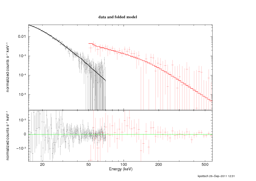
Finally, we check the source signal using low backgrounds.
XSPEC12>cornorm 1 -0.03 2 -0.015
 Spectrum 1 correction norm set to -0.03
 Spectrum 2 correction norm set to -0.015

 Chi-Squared =         911.15 using 197 PHA bins.
 Reduced chi-squared =         4.6967 for    194 degrees of freedom
 Null hypothesis probability =   2.974284e-93
 Current data and model not fit yet.
XSPEC12>fit
                    Parameters
Chi-Squared  Lvl          1:nH    2:PhoIndex        3:norm
808.384       -2       181.269       2.90266       1.54819
791.667       -2       174.773       2.84250       1.27043
772.645       -2       163.596       2.78155       1.03599
<more trials here>
434.587        0    0.00136529       1.83006     0.0445789
434.575        0   0.000110466       1.83001     0.0445767
434.575        6   0.000111649       1.83001     0.0445767
========================================
 Variances and Principal Axes
                 1        2        3
 1.4396E-07| -0.0000  -0.1354   0.9908
 1.4928E+02| -1.0000  -0.0006  -0.0001
 7.6104E-04| -0.0006   0.9908   0.1354
----------------------------------------

====================================
  Covariance Matrix
        1           2           3
   1.493e+02   8.576e-02   1.659e-02
   8.576e-02   7.964e-04   1.116e-04
   1.659e-02   1.116e-04   1.593e-05
------------------------------------

========================================================================
Model phabs<1>*powerlaw<2> Source No.: 1   Active/On
Model Model Component  Parameter  Unit     Value
 par  comp
   1    1   phabs      nH         10^22    1.11649E-04  +/-  12.2180
   2    2   powerlaw   PhoIndex            1.83001      +/-  2.82200E-02
   3    2   powerlaw   norm                4.45767E-02  +/-  3.99093E-03
________________________________________________________________________


 Chi-Squared =         434.58 using 197 PHA bins.
 Reduced chi-squared =         2.2401 for    194 degrees of freedom
 Null hypothesis probability =   1.748499e-20
XSPEC12>plot ldata res
The result is shown in 5.3 where now the GSO spectrum is largely above to model.
By comparing the different fit results from these different runs, the overall uncertainties expected for the slope and normalization can be estimated.
Xissim is a Suzaku XIS event simulator, based on the tool xrssim. It reads a FITS format photon list file, traces photon paths in the telescope (via ray-tracing), and outputs a simulated XIS event file. The XRT thermal shield transmission and the XIS detection efficiency are taken into account if requested. Each record of the photon list file describes the celestial positions, arrival time, and energy of the input photon. The mkphlist FTOOL can create such photon list files from FITS images (e.g., ROSAT HRI or Chandra images) and spectral models (which may be created in XSPEC). The xissim output event file may be analyzed just like observational data, using standard analysis tools such as xselect. xissim is part of the latest version of the FTOOLS.
Maki is another web-based interactive tool (see Appendix B) that can determine the orientation of the XIS CCDs on the sky as a function of the observation epoch within the visibility window of the target. For Suzaku, the orientation of the solar panels with respect to the spacecraft is fixed, and at the same time, the range of the angles between the vector normal to the solar panels and the vector pointing to the Sun is restricted, which in turn restricts the roll angle of the spacecraft.
When using the tool, general instructions are available via the ``Help'' button. In order to check the visibility and available roll angles for a target, load a FITS image or by enter the RA and DEC of the source and click the ``New Graph'' button. This creates an image on which the Suzaku XIS field of view (FOV) will be shown.
The ``Mission and Roll Selector'' (in the upper right of the display) allows different instruments from different missions to be selected. Then the FOV will appear on your image. This can be rotated using the ``Roll angle'' slider bar.
Unfortunately, the current version of Maki does not work on
64-bit machines. We therefore provide a simpler, text-only, perl
script, RollRange, as an alternative to Maki. The
RollRange package can be downloaded
from:
ftp://heasarc.gsfc.nasa.gov/suzaku/nra_info/tools/rollrange.tar.gz.
For
setup instructions, see:
http://heasarc.gsfc.nasa.gov/docs/suzaku/prop_tools/rollrange.html.
RollRange.pl
takes three arguments: the right ascension and declination of the
pointing direction in decimal degrees, and the MJD of interest (which
can be calculated using the HEASARC xTime tool).
At a roll angle of 0.0, the spacecraft's Y axis is pointing North; at 90.0, it points East (i.e., counterclockwise rotation looking up at the sky). One can subtract the roll angle from 90.0 to obtain the 3rd Euler angle.
Note that both Maki and RollRange consider only the Sun angle. Additional constraints often exist, due to the availability (or not) of suitable stars in the star-tracker field-of-view. For accepted observations, the mission scheduling team will provide the definitive range of allowed roll angles to the PI.
The Remote Proposal Submission (RPS) tool must be used to enter the basic proposal data into the ISAS/JAXA, HEASARC, or ESA database. Proposers should make sure they use the appropriate RPS, since there are multiple reviews. See Appendix B for the list of RPS web-sites and addresses. Two versions of RPS are available: a character-oriented version, where the user submits all the required information via e-mail, or a web-oriented version.
One aspect of RPS that is not immediately obvious is how to specify time-constrained observations. For instance, a need for such an observation may arise for a study of a spectrum of a binary system at a particular orbital phase. If some particular aspect of the observation cannot be clearly specified in the RPS form, the user should detail it in the ``comments'' field of the RPS form and/or contact either the Suzaku team at ISAS/JAXA or the NASA Suzaku GOF before submitting.
A successful Suzaku proposal, from a technical point of view, must include the following elements:
While two default aim points were offered from AO-1 to AO-6 -- the
XIS nominal and the HXD nominal positions (the HXD aim point is at
(DETX,DETY)=(-3.![]() 5, 0) on the XIS image); the reduction in
effective area for the non-selected instrument is
5, 0) on the XIS image); the reduction in
effective area for the non-selected instrument is ![]() %) --
support for the HXD nominal position will be dropped in AO-7. This is
done to mitigate effects due to the increased attitude jitter of Suzaku
since the end of 2009. No observations with non-standard readout clocks
(P-sum/Timing mode and Window/Burst options) will be carried out at
the HXD nominal position. While the operation team does not prohibit
observations at the HXD nominal point with a standard XIS mode
response matrices will not be provided for such observations.
%) --
support for the HXD nominal position will be dropped in AO-7. This is
done to mitigate effects due to the increased attitude jitter of Suzaku
since the end of 2009. No observations with non-standard readout clocks
(P-sum/Timing mode and Window/Burst options) will be carried out at
the HXD nominal position. While the operation team does not prohibit
observations at the HXD nominal point with a standard XIS mode
response matrices will not be provided for such observations.
Note that Guest Observers are welcome to propose for targets already approved for in previous AOs (see the Announcement of Opportunity). However, in the interest of maximizing the scientific return from Suzaku, the proposal must explain why the already-approved observation(s) does/do not meet their scientific objectives. Valid reasons include a much longer exposure time, incompatible time constraints, or different positions within an extended source.
We also note that the XISs are subject to count rate limitations,
because of possible multiple events in an XIS pixel within one
frame. This is much less of a problem than with the ACIS aboard
Chandra, as Chandra's mirror focuses the X-ray flux onto a CCD area
that is orders of magnitude smaller. The rule of thumb is that the XIS
can tolerate a point source with a count rate up to ![]() cps per
CCD with essentially no loss of counts or resolution. For brighter
sources, these limitations can be reduced via a variety of XIS modes,
such as the use of a sub-array of the XIS, as discussed in
section 7.2.2.1.
cps per
CCD with essentially no loss of counts or resolution. For brighter
sources, these limitations can be reduced via a variety of XIS modes,
such as the use of a sub-array of the XIS, as discussed in
section 7.2.2.1.
Finally, it is important to remember that because the HXD is a
non-imaging detector, contaminating sources in the field of view can
significantly affect your results. The HXD field of view is defined by
a collimator with a square opening. The FWHM of the field of view is
34.![]() 4
4 ![]() 34.
34.![]() 4 below
4 below ![]() keV and
keV and
![]() above
above ![]() keV. Considering that twice the
FWHM value is required to completely eliminate the contamination in a
collimator-type detector, and the source may happen to be located at
the diagonal of the square, nearby bright sources within a radius of
50
keV. Considering that twice the
FWHM value is required to completely eliminate the contamination in a
collimator-type detector, and the source may happen to be located at
the diagonal of the square, nearby bright sources within a radius of
50![]() and
and ![]() from the aim point can contaminate the
data in the energy band below and above
from the aim point can contaminate the
data in the energy band below and above ![]() keV, respectively.
If you specify the roll-angle to avoid the source, the limit will be
reduced to
keV, respectively.
If you specify the roll-angle to avoid the source, the limit will be
reduced to ![]() 35
35![]() and
and
![]() , respectively. It
is the proposer's responsibility to show that any source with a flux
level comparable to or brighter than that of the target of interest
does not exist within these ranges. The proposer can, e.g., check this
by using the hard X-ray source catalogs from such satellites as
RXTE-ASM, INTEGRAL, and Swift, among
others.
, respectively. It
is the proposer's responsibility to show that any source with a flux
level comparable to or brighter than that of the target of interest
does not exist within these ranges. The proposer can, e.g., check this
by using the hard X-ray source catalogs from such satellites as
RXTE-ASM, INTEGRAL, and Swift, among
others.
There are two additional NASA-specific proposal rules that must be followed by US-based proposers: