7. An EPIC Data Processing and Analysis Primer

While a variety of analysis packages can be used for the following steps, the SAS was designed for the basic reduction and analysis of XMM-Newton data (extraction of spatial, spectral, and temporal data); therefore, it will be used here for demonstration purposes.

NOTE: For PN observations with very bright sources, out-of-time events can provide a serious contamination of the image. Out-of-time events occur because the read-out period for the CCDs can be up to $\sim6.3$% of the frame time. Since events that occur during the read-out period can't be distinguished from others events, they are included in the event files but have invalid locations. For observations with bright sources, this can cause bright stripes in the image along the CCD read-out direction.

At this point, it is assumed that you have downloaded the data from the HEASARC archive onto a Hera server, standard or anonymous Hera is running (see §4.2), and you have prepared the data for processing (see §6). Throughout this chapter, as in §6, we will use the Lockman Hole dataset with ObsID 0123700101, though any dataset will suffice.

7.1 Rerun the Pipeline

If a dataset is more than a year old, it was probably processed with older versions of CCF and SAS prior to archiving, so the pipeline should be rerun to generate event files with the latest calibrations. The MOS has two pipeline tasks, emchain and emproc, while the PN has one, epproc for the PN. The two MOS tasks produce the same output, so which one to use is entirely a matter of the user's personal preference.

Verify that the working directory PROC is highlighted in the GUI. In the new Command Window you made at the end of §6, run the task(s):

emchain

or

emproc

and

epproc

If the dataset has more than one exposure, a specific exposure can be accessed using the exposure parameter, e.g.:

emchain exposure=n

where n is the exposure number. To create an out-of-time event file for your PN data, add the parameter withoutoftime to your epproc invocation:

epproc withoutoftime=yes

By default, none of these tasks keep any intermediate files they generate. Emchain maintains the naming convention described in §5.3.3. Emproc and epproc designate their output event files with ``Evts.ds''; ``*ImagingEvts.ds'', ``*TimingEvts.ds'', and ``*BurstEvts.ds'' denote the imaging mode, timing, and burst mode event lists, respectively. In either case, you may want to name the new files something easy to type. Right-clicking on a file will give you the option to rename it.

Once the new event files have been obtained, the analysis techniques described below can be used. We will refer to the new event files as mos1.fits, mos2.fits, and pn.fits.

7.2 Examine and Analyze Data

7.2.1 Create and Display an Image

To create an image in sky coordinates, type

evselect table=mos1.fits withimageset=yes imageset=image.fits
$$ xcolumn=X ycolumn=Y imagebinning=imageSize ximagesize=600 yimagesize=600

where

table - input event table
withimageset - make an image
imageset - name of output image
xcolumn - event column for X axis
ycolumn - event column for Y axis
imagebinning - form of binning, force entire image into a given size or bin by a specified number of pixels
ximagesize - output image pixels in X
yimagesize - output image pixels in Y

The resultant image is written to the file image.fits. It can be viewed with POW, or downloaded to your local machine and viewed with ds9; see Figure 7.1.

Figure 7.1: The MOS1 image, displayed in fv.

7.2.2 Create and Display a Light Curve

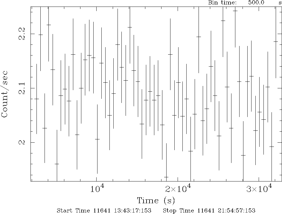
To create a light curve, type

evselect table=mos1.fits withrateset=yes rateset=mos1_ltcrv.fits
$$ maketimecolumn=yes timecolumn=TIME timebinsize=100 makeratecolumn=yes

where

table - input event table
withrateset - make a light curve
rateset - name of output light curve file
maketimecolumn - control to create a time column
timecolumn - time column label
timebinsize - time binning (seconds)
makeratecolumn - control to create a count rate column, otherwise a count column will be created

The output file mos1_ltcrv.fits can be viewed with POW; see Fig. 7.2.

Figure 7.2: The light curve.

7.2.3 Applying Standard Filters the Data

The filtering expressions for the MOS and PN are:

(PATTERN $<=$ 12)&&(PI in [200:12000])&&#XMMEA_EM

and

(PATTERN $<=$ 12)&&(PI in [200:15000])&&#XMMEA_EP

If the PN data is timed, then the PATTERN parameter should be set to 4:

(PATTERN $<=$ 4)&&(PI in [200:15000])&&#XMMEA_EP.

The first two expressions will select good events with PATTERN in the 0 to 12 range, and the last will select events with PATTERN between 0 and 4. The PATTERN value is similar the GRADE selection for ASCA data, and is related to the number and pattern of the CCD pixels triggered for a given event.The PATTERN assignments are: single pixel events: PATTERN == 0, double pixel events: PATTERN in [1:4], triple and quadruple events: PATTERN in [5:12].

The second keyword in the expressions, PI, selects the preferred pulse height of the event; for the MOS, this should be between 200 and 12000 eV. For the PN, this should be between 200 and 15000 eV. This should clean up the image significantly with most of the rest of the obvious contamination due to low pulse height events. Setting the lower PI channel limit somewhat higher (e.g., to 300 eV) will eliminate much of the rest.

Finally, the #XMMEA_EM (#XMMEA_EP for the PN) filter provides a canned screening set of FLAG values for the event. (The FLAG value provides a bit encoding of various event conditions, e.g., near hot pixels or outside of the field of view.) Setting FLAG == 0 in the selection expression provides the most conservative screening criteria and should always be used when serious spectral analysis is to be done on the PN.

It is a good idea to keep the output filtered event files and use them in your analyses, as opposed to re-filtering the original file with every task. This will save much time and computer memory. As an example, the Lockman Hole data's original event file is 48.4 Mb; the fully filtered list (that is, filtered spatially, temporally, and spectrally) is only 4.0Mb!

To filter the data, type

evselect table=mos1.fits withfilteredset=yes
$$ expression='(PATTERN $<=$ 12)&&(PI in [200:12000])&&#XMMEA_EM'
$$ filteredset=mos1_filt.fits filtertype=expression keepfilteroutput=yes
$$ updateexposure=yes filterexposure=yes

where

table - input event table
filtertype - method of filtering
expression - filtering expression
withfilteredset - create a filtered set
filteredset - output file name
keepfilteroutput - save the filtered output
updateexposure - for use with temporal filtering
filterexposure - for use with temporal filtering

7.2.4 Applying Time Filters the Data

Sometimes, it is necessary to use filters on time in addition to those mentioned above. This is because of soft proton background flaring, which can have count rates of 100 counts/sec or higher.

It should be noted that the amount of flaring that needs to be removed depends in part on the object observed; a faint, extended object will be more affected than a very bright X-ray source.

There are two ways to filter on time: with an explicit reference to the TIME or RATE parameters in the filtering expression, or by creating a secondary Good Time Interval (GTI) file with the task tabgtigen. Both procedures are described below. For the example data, we will filter by time, though you can just as easily filter by rate.

To explicitly define the TIME or RATE parameters, make a light curve and display it, as demonstrated in §7.2.2 and plotted in Figure 7.2. There is a very large flare toward the end of the observation, so the syntax for the time selection is (TIME $<=$ 7.32273e7). However, there is also a small flare within an otherwise good interval. A slightly more comlicated expression to remove it would be: (TIME $<=$ 7.32273e7)&&!(TIME IN [7.32219e7:7.32238e7]). The syntax &&(TIME $<$ 7.32273e7) includes only events with times less than 7.32273e7, and the ``!'' symbol stands for the logical ``not'', so use &&!(TIME in [7.32219e7:7.32238e7]) to exclude events in the time interval 7.32219e7 to 7.32238e7.

If combined with the standard filtering expression (see §7.2.3), the full filtering expression would then be:

(PATTERN $<=$ 12)&&(PI in [200:12000])&&#XMMEA_EM
$$ &&(TIME $<=$ 7.32273e7) &&!(TIME in [7.32219e7:7.32238e7])

This expression can then be used to filter the original event file, as shown in §7.2.3, or only the times can be used to filter the file that has already had the standard filters applied:

evselect table=mos1_filt.fits withfilteredset=yes
$$ expression='(TIME $<=$ 7.32273e7) &&!(TIME in [7.32219e7:7.32238e7]) '
$$ filteredset=mos1_filt_time.fits filtertype=expression keepfilteroutput=yes
$$ updateexposure=yes filterexposure=yes

where the keywords are as described in §7.2.3.

To filter on time using a secondary GTI file, make the file by using the same time filtering parameters as determined above and the tabgtigen task,

tabgtigen table=mos1_ltcrv.fits gtiset=gtiset.fits timecolumn=TIME
$$ expression='(TIME $<=$ 7.32273e7) &&!(TIME in [7.32219e7:7.32238e7])'

where

table - input count rate table
expression - filtering expression
gtiset - output file name for selected GTI intervals
timecolumn - time column

and apply the new GTI file with the evselect task:

evselect table=mos1_filt.fits withfilteredset=yes
$$ expression='GTI(gtiset.fits,TIME)' filteredset=mos1_filt_time.fits
$$ filtertype=expression keepfilteroutput=yes
$$ updateexposure=yes filterexposure=yes

where

table - input count rate table
expression - filtering expression
withfilteredset - create a filterered set
filteredset - output file name
filtertype - method of filtering
keepfilteroutput - save the filtered set
updateexposure - update exposure information in event list and in spectrum files
filterexposure - filter exposure extensions of event list with same time
$$ filters as for corresponding CCD

7.2.5 Source Detection with edetect_chain

The task edetect_chain is a metatask that does nearly all the work involved with EPIC source detection. It can take as input arbitrary combinations of images from different energy bands and different EPIC instruments, with up to three instruments and 5 energy bands. However, users should be aware that that the binning and WCS keywords in all images must be identical. Edetect_chain is comprised of seven straightforward tasks that can also be run by hand. Edetect_chain requires input files to be generated and prepared using the tasks atthkgen and evselect; the task emosaic, while not necessary for source detection, does provide a nice mosaicked image for display purposes. Fortunately, these are all quick and straightforward.

In the example below, source detection on images is done in two bands, 500 - 1000 eV and 4500 - 12000 eV, which correspond to bands 2 and 5 of the 3XMM Catalogue, for all three detectors. The source count rates are converted into fluxes through the energy converstion factors (ECFs) for each detector and energy band. The ECFs depend on the pattern selection and filter used during the observation and are given in units of $10^{11}$ cts cm$^{2}$/erg. Interested users can find all of the bands listed in Table 1 of the Catalogue. The ECFs are in Table 8 of the Catalogue.)

The example uses the filtered event files from all three cameras, which can be produced in §7.2.4.

First, make the attitude file:

atthkgen atthkset=attitude.fits timestep=1

where

atthkset - output file name
timestep - time step in seconds for attitude file

Next, make the band 2 and band 5 images with evselect. We'll start with the band 2 image in the MOS1.

evselect table=mos1_filt_time.fits withimageset=yes imageset=mos1-b2.fits
$$ imagebinning=binSize xcolumn=X ximagebinsize=82 ycolumn=Y yimagebinsize=82
$$ filtertype=expression expression='(FLAG == 0)&&(PI in [500:1000])'

and

evselect table=mos1_filt_time.fits withimageset=yes imageset=mos1-b5.fits
$$ imagebinning=binSize xcolumn=X ximagebinsize=82 ycolumn=Y yimagebinsize=82
$$ filtertype=expression expression='(FLAG == 0)&&(PI in [4500:12000])'

The procedure is similar for the MOS2 and PN. Note that, because we are using these images for the specific purpose of source detection, the image binning that we would normally use for MOS (22, corresponding to 1.1 arcsec) must be adjusted to match that of PN (82, corresponding to 4.1 arcsec). For the band 5 images, set the ``Selection Expression'' text to (FLAG == 0)&&(PI in [4500:12000]). We will assume the output images are named mos1-b2.fits, mos2-b2.fits, pn-b2.fits, mos1-b5.fits, mos2-b5.fits, and pn-b5.fits.

Now we can run edetect_chain:

edetect_chain
$$ imagesets='mos1-b2.fits mos1-b5.fits mos2-b2.fits mos2-b5.fits pn-b2.fits pn-b5.fits'
$$ eventsets='mos1_filt_time.fits mos2_filt_time.fits pn_filt_time.fits'
$$ attitudeset=attitude.fits likemin=10 witheexpmap=yes
$$ pimin='500 4500 500 4500 500 4500' pimax='1000 12000 1000 12000 1000 12000'
$$ ecf='1.70 0.15 1.71 0.15 7.87 0.58' eboxl_list=eboxlist_l.fits
$$ eboxm_list=eboxlist_m.fits eml_list=emllist.fits esp_withootset=no

where

imagesets - list of count images
eventsets - list of event files
attitudeset - attitude file name
pimin - list of minimum PI channels for the bands
pimax - list of maximum PI channels for the bands
likemin - maximum likelihood threshold
witheexpmap - create and use exposure maps
ecf - energy conversion factors for the bands
eboxl_list - output file name for the local sliding box source
$$ detection list
eboxm_list - output file name for the sliding box source detection in
$$ background map mode list
eml_list - output file name for maximum likelihood source detection list
esp_withootset - Flag to use an out-of-time processed PN event file,
$$useful in cases where bright point sources have left streaks in the PN data
esp_ooteventset - The out-of-time processed PN event file

7.2.6 Extract the Source and Background Spectra

Throughout the following, please keep in mind that some parameters are instrument-dependent. The parameter specchannelmax should be set to 11999 for the MOS, or 20479 for the PN. Also, for the PN, the most stringent filters, (FLAG==0)&&(PATTERN<=4), must be included in the expression to get a high-quality spectrum.

For the MOS, the standard filters should be appropriate for many cases, though there are some instances where tightening the selection requirements might be needed. For example, if obtaining the best-possible spectral resolution is critical to your work, and the corresponding loss of counts is not important, only the single pixel events should be selected (PATTERN==0). If your observation is of a bright source, you again might want to select only the single pixel events to mitigate pile up (see §7.2.8 and §7.2.9 for a more detailed discussion).

First, make an image of the filtered file, mos1_filt_time.fits, as described in §7.2.1). Download it and display it with ds9, then click on an object whose spectrum you wish to extract. Adjust the extraction region until you are satisfied with it. For this example, we will choose the source at (26165.75, 22816.25) and set the extraction radius to 400.

To extract the source spectrum, type

evselect table='mos1_filt_time.fits' energycolumn='PI' withfilteredset=yes
$$ filteredset='mos1_filt_time_source.fits' keepfilteroutput=yes filtertype='expression'
$$ expression='((X,Y) in CIRCLE(26165.75,22816.2,400))&&(FLAG==0)'
$$ withspectrumset=yes spectrumset='mos1_source_pi.fits' spectralbinsize=5
$$ withspecranges=yes specchannelmin=0 specchannelmax=11999

where

table - the event file
energycolumn - energy column
withfilteredset - make a filtered event file
keepfilteroutput - keep the filtered file
filteredset - name of output file
filtertype - type of filter
expression - expression to filter by
withspectrumset - make a spectrum
spectrumset - name of output spectrum
spectralbinsize - size of bin, in eV
withspecranges - covering a certain spectral range
specchannelmin - minimum of spectral range
specchannelmax - maximum of spectral range

The spectrum, in counts per channel, can be viewed with fv.

When extracting the background spectrum, follow the same procedures, but change the extraction area. For example, make an annulus around the source; this can be done using two circles, each defining the inner and outer edges of the annulus, then change the filtering expression (and output file name) as necessary.

To extract the background spectrum, type

evselect table='mos1_filt_time.fits' energycolumn='PI' withfilteredset=yes
$$ filteredset='mos1_filt_time_bkg.fits' keepfilteroutput=yes filtertype='expression'
$$ expression='((X,Y) in CIRCLE(26165.75,22816.2,1200))&&!((X,Y) in CIRCLE(26165.75,22816.2,400))'
$$ withspectrumset=yes spectrumset='mos1_bkg_pi.fits' spectralbinsize=5
$$ withspecranges=yes specchannelmin=0 specchannelmax=11999

where the keywords are as described above.

7.2.7 Determine the Spectrum Extraction Areas

The source and background region areas can now be found. This is done with the task backscale, which takes into account any bad pixels or chip gaps, and writes the result into the BACKSCAL keyword of the spectrum table.

To find the source and background extraction areas, type

backscale spectrumset=mos1_source_pi.fits badpixlocation=mos1_filt_time.fits

and

backscale spectrumset=mos1_bkg_pi.fits badpixlocation=mos1_filt_time.fits

7.2.8 Check for Pile Up

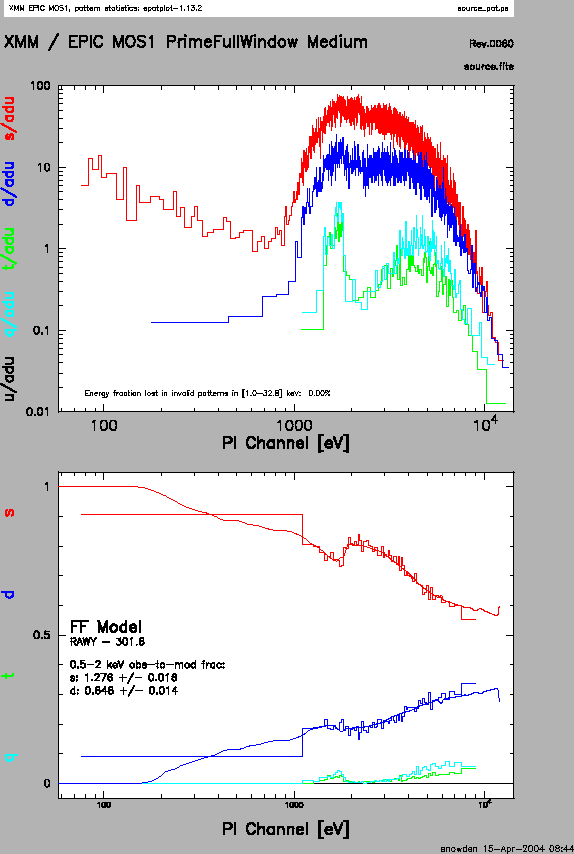
Depending on how bright the source is and what modes the EPIC detectors are in, event pile up may be a problem. Pile up occurs when a source is so bright that incoming X-rays strike two neighboring pixels or the same pixel in the CCD more than once in a read-out cycle. In such cases the energies of the two events are in effect added together to form one event. If this happens sufficiently often, 1) the spectrum will appear to be harder than it actually is, and 2) the count rate will be underestimated, since multiple events will be undercounted. To check whether pile up may be a problem, use the SAS task epatplot. (Heavily piled sources will be immediately obvious, as they will have a ``hole'' in the center.) Note that this procedure requires as input the event files created when the spectrum was made.

The output of epatplot is a postscript file, which may be viewed with viewers such as gv, containing two graphs describing the distribution of counts as a function of PI channel; see Figure 7.3.

A few words about interpretting the plots are in order. The top is the distribution of counts versus PI channel for each pattern class (single, double, triple, quadruple), and the bottom is the expected pattern distribution (smooth lines) plotted over the observed distribution (histogram). If the lower plot shows the model distributions for single and double events diverging significantly from the observed distributions, then the source is piled up.

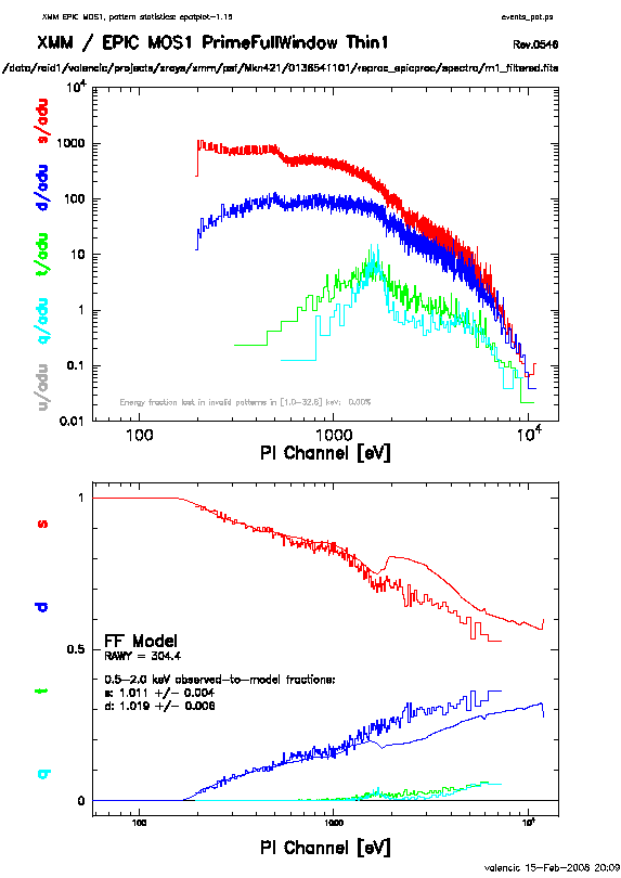
The source used in our Lockman Hole example is too faint to provide reasonable statistics for epatplot and is far from being affected by pile up. In contrast, plots from two different observations are shown in Figure 7.3 and 7.4. In Figure 7.3, the source is bright enough to provide statistics (and a good fit) at energies above about 1.5 keV. Figure 7.4 shows a plot of a very bright source which is strongly affected by pileup. Note the severe divergence between the model and the observed pattern distribution.

To check for pile up, type

epatplot set=mos1_filt_time_source.fits plotfile=mos1_pat.ps
$$ useplotfile=yes withbackgroundset=yes backgroundset=mos1_filt_time_bkg.fits

The postscript file can be copied to the user's local machine and viewed there.

Figure 7.3: The output of epatplot for a source without pileup. Note that in the lower plot, for energies less than $\sim$ 1500 eV, there are too few X-rays for epatplot to model.

Figure 7.4: The output of epatplot for a heavily piled source. In the lower plot, there are large differences between the predicted and observed pattern distribution at energies above $\sim$ 1000 eV.

7.2.9 My Observation is Piled Up! Now What?

There are a few ways to deal with pile up. First, using the region selection and event file filtering procedures demonstrated in earlier sections, you can excise the inner-most regions of a source (as they are the most heavily piled up), re-extract the spectrum, and continue your analysis on the excised event file. For this procedure, it is recommended that you take an iterative approach: remove an inner region, extract a spectrum, check with epatplot, and repeat, each time removing a slightly larger region, until the model and observed distribution functions agree.

You can also use the event file filtering procedures to include only single pixel events (PATTERN==0), as these events are less sensitive to pile up than other patterns.

7.2.10 Create the Photon Redistribution Matrix (RMF) and Ancillary File (ARF)

In order to do spectral analysis, it is necessary to find the instrument's repsonse as a function of energy and PI channel. This is done by reformating the detector response and energy bounds information and correcting for instrumental effects, and writing the result to the Redistribution Matrix File (RMF). The following assumes that an appropriate source spectrum, named mos1_source_pi.fits, has been extracted as in §7.2.6.

To make the RMF, type

rmfgen rmfset=mos1_rmf.fits spectrumset=mos1_source_pi.fits

where

rmfset - output file
spectrumset - spectrum file

Now use the RMF, spectrum, and event file to make the ancillary file.

To make the ARF, type

arfgen arfset=mos1_arf.fits spectrumset=mos1_source_pi.fits withrmfset=yes
$$ rmfset=mos1_rmf.fits withbadpixcorr=yes badpixlocation=mos1_filt_time.fits

where

arfset - output ARF file name
spectrumset - input spectrum file name
withrmfset - flag to use the RMF
rmfset - RMF file created by rmfgen
withbadpixcorr - flag to include the bad pixel correction
badpixlocation - file containing the bad pixel information; should be set to the event
$$ file from which the spectrum was extracted.

At this point, the spectrum is ready to be analyzed, so we can prepare the spectrum for fitting.

7.2.11 Prepare and Fit the Spectrum

With the source and background spectra now extracted and the RMF and ARF created, we will do some simple spectral fitting. SAS does not include fitting software, so HEASoft packages will be used, and all fitting tasks will be called from the Command Window.

Nearly all spectra will need to be binned for statistical purposes. The procedure grppha, located in the HEASARC folder in the Available Tools window, provides an excellent mechanism to do just that.

The following commands not only group the source spectrum for Xspec but also associate the appropriate background and response files for the source.

1)

In the Command Window, type:

grppha

and edit the parameters and file names as appropriate:

      Please enter PHA filename[] mos1_source_pi.fits ! input spectrum file name
      Please enter output filename[] mos1_grp.fits    ! output grouped spectrum
      GRPPHA[] chkey BACKFILE mos1_bkg_pi.fits        ! include the background spectrum
      GRPPHA[] chkey RESPFILE mos1_rmf.fits           ! include the RMF
      GRPPHA[] chkey ANCRFILE mos1_arf.fits           ! include the ARF
      GRPPHA[] group min 25                           ! group the data by 25 counts/bin
      GRPPHA[] exit

Upon exiting, the output file mos1_grp.fits will appear in your working directory.

Next, use Xspec to fit the spectrum by typing:

xspec

A POW window will pop up and display the spectrum later on. Edit the parameters and file names as appropriate:

      XSPEC> data mos1_grp.fits      ! input data
      XSPEC> ignore 0.0-0.2,6.6-**   ! ignore unusable energy ranges, in keV
                                     ! set a range appropriate for the data
      XSPEC> model wabs(pow+pow)     ! set spectral model to two absorbed power laws
      1:wabs:nH> 0.01                ! set model absorption column density to 1.e20
      2:powerlaw:PhoIndex> 2.0       ! set the first model power law index to -2.0
      3:powerlaw:norm>               ! use the default model normalization
      4:powerlaw:PhoIndex> 1.0       ! set the second model power law index to -1.0
      5:powerlaw:norm>               ! use the default model normalization
      renorm                         ! renormalize the model spectrum
      XSPEC> fit                     ! fit the model to the data
      XSPEC> setplot energy          ! plot energy along the X axis
      XSPEC> plot ldata ratio        ! plot two panels with the log of the data and
                                     !     the data/model ratio values along the Y axes
      XSPEC> exit                    ! exit Xspec

Figure 7.5 shows the fit to the spectrum.

Figure 7.5: The fitted spectrum of the Lockman Hole source.

7.3 Timing Analysis

This section will demonstrate some basic timing analysis of EPIC image-mode data using the Xronos analysis package. For this exercise, the central source from the observation of G21.5-09 (Obs ID 0122700101) is used. These examples assume that the source's lightcurve has been made as in §7.2.2, but with timebinsize set to 1 and makeratecolumn set to no; the name of this file assumed to be source_ltcrv.fits.

For the aficionado, the task barycen can be used for the barycentric correction of the source event arrival times.

The Xronos tools can be access through Hera by clicking on XRONOS in the Available Tools panel.

Figure 7.6: Light curve for the source analyzed as in §7.2.2.

Figure 7.7: Power spectrum density for the source.

To make a binned lightcurve, type:

lcurve nser=1 cfile1='source_ltcrv.fits' window=- dtnb=500 nbint=450
$$ outfile='lightcurve_binned.fits' plot=no

where

nser - number of time series
cfile1 - filename first series
window - name of window file (if a subset of the time series is required)
dtnb - bin size (time)
nbint - number of bins per interval
outfile - output file name (FITS format light curve)
plot - plot flag

The output can be viewed with fv by right-clicking on the filename and selecting the ``Edit/Display File'' option. Output is shown in Figure 7.6.

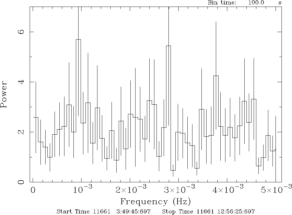
To calculate power spectrum density, type

powspec cfile1='source_ltcrv.fits' window=- dtnb=100.0 nbint=300
$$ nintfm=INDEF rebin=5 plot=no outfile='power.fits'

where

cfile1 - filename first series
window - name of window file (if a subset of the time series is required)
dtnb - bin size (time)
nbint - number of bins per interval
nintfm - number of intervals in each power spectrum
rebin - rebin factor for power spectrum (0 for no rebinning)
plot - plot flag
outfile - output file name (FITS format power spectrum)

The output can be viewed with fv by right-clicking on the filename and selecting the ``Edit/Display File'' option. Output is shown in Figure 7.7.

To search for periodicities in the time series, type:

efsearch cfile1=source_ltcrv.fits window=- sepoch=INDEF dper=20 nphase=10
$$ nbint=INDEF nper=100 dres=INDEF plot=no outfile=autocor.fits

where

cfile1 - filename first series
window - name of window file (if a subset of the time series is required)
sepoch - value for epoch used for phase zero when folding the time series
dper - value for the period used in the folding
nphase - number of phases per period
nbint - number of bins per interval
nper - number of sampled periods during search
dres - sampling resolution of search
plot - plot flag
outfile - output file name (FITS format)

To calculate the autocorrelation for a time series, type:

autocor cfile1=source_ltcrv.fits window=- dtnb=24.0 nbint=2048 nintfm=INDEF
$$ rebin=0 plot=no outfile=auto.fits

where

cfile1 - filename first series
window - name of window file (if a subset of the time series is required)
dtnb - bin size (time)
nbint - number of bins per interval
nintfm - number of intervals to be summed in each autocorrelation function
rebin - rebin factor for autocorrelation function (0 for no rebinning)
plot - plot flag
outfile - output file name (FITS format autocorrelation spectrum)

To calculate statistical quantities for a time series, type

lcstats cfile1=source_ltcrv.fits window=- dtnb=6.0 nbint=8192

where

cfile1 - filename first series
window - name of window file
dtnb - integration time (binning)
nbint - number of bins

The output will be written in the Command Window.