Next: Notes on Normalization Up: Running XSTAR2XSPEC Previous: Output Contents
If you are using mtables with variable abundances, then you will likely get totally unphysical results unless you note the following.
The mtable models are constructed using two kinds of parameters: interpolated
parameters and additive parameters. Interpolated parameters are treated
as one might expect: if the model is represented by a vector ![]() ,
corresponding to the model flux at various energies
,
corresponding to the model flux at various energies ![]() and
stored at various values of the free (intepolated) parameter
and
stored at various values of the free (intepolated) parameter ![]() ,
then for a value of the parameter not on the tabulated grid xspec
calculates the model value as
,
then for a value of the parameter not on the tabulated grid xspec
calculates the model value as
where ![]() are suitably chosen weights for, eg. linear
interpolation. Ths is in contrast to the treatment of additive parameters:
for an mtable, xspec needs the value of the model tabulated at only
two values of the free additive parameter
are suitably chosen weights for, eg. linear
interpolation. Ths is in contrast to the treatment of additive parameters:
for an mtable, xspec needs the value of the model tabulated at only
two values of the free additive parameter ![]() , 0 and
, 0 and ![]() . Then the
model is calculated for some arbitrary
. Then the
model is calculated for some arbitrary ![]() as
as
i.e. it is assumed that the model scales linearly with the value
of the additive parameter ![]() . This formalism was developed for
emission models, where emissivities might be expected to scale
linearly with elemental abundance. In the case of absorption models,
the value of
. This formalism was developed for
emission models, where emissivities might be expected to scale
linearly with elemental abundance. In the case of absorption models,
the value of ![]() which xspec uses is a transmission coefficient, and this
does not scale linearly with abundance. Rather, the transmission coefficient
is related to the optical depth by:
which xspec uses is a transmission coefficient, and this
does not scale linearly with abundance. Rather, the transmission coefficient
is related to the optical depth by:
and the optical depth ![]() does scale (approximately) linearly
with abundance. For this reason, xspec has incorporated the etable models,
in which the model builder supplies optical depths rather than transmission
coefficient, linear interpolation is used to calculate the optical depth
for a given abundance, and then the transmission coefficient is
calculated using the above expression. The results:
does scale (approximately) linearly
with abundance. For this reason, xspec has incorporated the etable models,
in which the model builder supplies optical depths rather than transmission
coefficient, linear interpolation is used to calculate the optical depth
for a given abundance, and then the transmission coefficient is
calculated using the above expression. The results:
(1) If you use an mtable calculated by xstar2xspec using varable abundances
(i.e. any additive parameters allowed to vary) in xspec using
the `model mtablexout_mtable.fits' command, you will get unphysical
results. It is easy to see that if ![]() is non-zero (which it often
is owing to 0 abundances) then you will never get deep absorption.
is non-zero (which it often
is owing to 0 abundances) then you will never get deep absorption.
(2) If so, you should use the `model etablexout_mtable2.fits' command in xspec instead. Entering parameter, etc., in xspec is the same for etables as for mtables.
(3) BUT, the etable itself is supposed to be filled with optical depths, not
transmission coefficients. The tables made by xstar2xspec are transmission coefficients,
and they need to be converted. This is a simple transformation: replace
the contents of every cell of the model extension of the mtable file (![]() )
with -ln(
)
with -ln(![]() ). This can be done various ways. One way is to use the calculator
inside of the ftools gui routine xv, one column at a time. This has
been done for the various precalculated models on the website, and these
are stored with the names xout_mtable2.fits.
). This can be done various ways. One way is to use the calculator
inside of the ftools gui routine xv, one column at a time. This has
been done for the various precalculated models on the website, and these
are stored with the names xout_mtable2.fits.
_________________________________________________________________________________
Some Specific Examples, and a Discussion of the Analytic Model warmabs
When fitting to absorption spectra it is important to be aware of the inherent limitations of xstar when applied to the fitting of absorption. There are two distinct reasons for this: spectral resolution effects, and interpolation effects. In order to illustrate these effects, we reproduce here a discussion between TK and P. Oneill of Imperial College in which these questions are raised, and some of the issues are discussed.
Question:
I've been using some of the sample XSPEC models from the current version of XSTAR to model a warm absorber.
I've been using the grid18 models with the abundances fixed at their default values. I found that using the XSPEC model "mtablexout_mtable.fits*powerlaw" gave different results (less absorption) than when I used "etablexout_mtable_2.fits*powerlaw". I thought that these should provide the same results, so long as the abundances are not changed. Am I using these tables correctly, or is there perhaps a problem somewhere?
Answer:
The problem is that variable abundances, they are treated as additive parameters in xspec tables, really can't be treated accurately using either type of table. If you use an mtable, then the transmittivity in a bin, i, at a given ionization parameter and column, is:
| (7.3) |
where ![]() is the 'zero abundance' version of the model at that
ionization parameter and column,
is the 'zero abundance' version of the model at that
ionization parameter and column, ![]() is the abundance of element j,
and
is the abundance of element j,
and ![]() is the model calculated with that element set to unity (relative
to cosmic). The first problem with this approach is that tranmission
doesn't scale this way with abundance. If you double the abundance
of an element, you should double the optical depth. Doubling the
transmittivity has both the wrong qualitative and quantitative behavior.
But an even bigger problem with this is that the whole thing,
is the model calculated with that element set to unity (relative
to cosmic). The first problem with this approach is that tranmission
doesn't scale this way with abundance. If you double the abundance
of an element, you should double the optical depth. Doubling the
transmittivity has both the wrong qualitative and quantitative behavior.
But an even bigger problem with this is that the whole thing, ![]() ,
multiplies your continuum. It is almost guaranteed to bigger than 1 if
some of the
,
multiplies your continuum. It is almost guaranteed to bigger than 1 if
some of the ![]() are non-zero. So this is totally the wrong formulation to
use when the abundances vary.
are non-zero. So this is totally the wrong formulation to
use when the abundances vary.
In the case of an etable the transmittivity is:
| (7.4) |
where
![]() etc.
etc.
This is better, since it predicts the correct dependence on abundance, i.e. that the optical depth scales approximately linearly with abundance.
But it is important to remember that what you are trying
to simulate is a 'real' photoionized gas with some abundance set ![]() that fits your data. What you are using to fit to your data are
that fits your data. What you are using to fit to your data are ![]() ,
which in the case of xstar are models calculated with only hydrogen and
helium, and the set of
,
which in the case of xstar are models calculated with only hydrogen and
helium, and the set of ![]() , which are supposed to be calculated with
pure element j.
, which are supposed to be calculated with
pure element j.
The first problem is that the cooling, and therefore the temperature, depends on the element abundance in the gas, and this is not linear. The temperature couples back into the ionization balance, and that affects the opacity, transmittivity, etc.
The second problem is that, while it is straightforward to calculate
a model with no elements heavier than H and He,
it is not straightforward to calculate a
model with pure iron, or calcium, say. That's because H and He havs nice
simple cooling properties at low temperature, and their opacity is simple,
etc. Pure iron models at best are likely to be very different than
H+He+Fe models, or from a cosmic mix. So what I do is make the ![]() using H+He+element j in cosmic ratios. But the problem with this is that
then the opacity due to H and He are present
in every
using H+He+element j in cosmic ratios. But the problem with this is that
then the opacity due to H and He are present
in every ![]() , and
, and ![]() ,
particularly at low ionization parameters. So if you sum over cosmic
abundances using an etable you are including the H and He opacity with
every one of the
,
particularly at low ionization parameters. So if you sum over cosmic
abundances using an etable you are including the H and He opacity with
every one of the ![]() . At high ionization parameter (log(
. At high ionization parameter (log(![]() 1?)
this
should not be a problem because H and He are ionized sufficiently that they do
not contribute to the opacity. But at low ionization parameter, the
model spectra calculated using etables will have significantly more
low energy opacity due to the multiple counting of H and He than they
would in a real xstar model with the corresponding parameters.
1?)
this
should not be a problem because H and He are ionized sufficiently that they do
not contribute to the opacity. But at low ionization parameter, the
model spectra calculated using etables will have significantly more
low energy opacity due to the multiple counting of H and He than they
would in a real xstar model with the corresponding parameters.
The strategy to use at low ionization parameters therefore is to use the etable to find a reasonably good fit to the spectrum with xspec, and then run xstar2xspec and make a very small table, i.e. just 1 column and 2 ionization parameters (xspec needs tables to have at least 2 entries), with constant abundances, set to the values which come from the fit. Constant abundance grids (such as grid19) when used as mtables do not suffer from any of these problems.
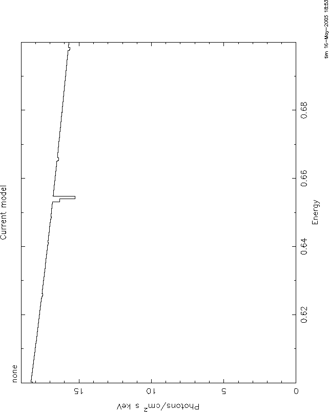
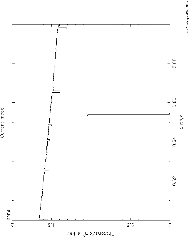
I attach 4 figures to illustrate these problems. All use the mtable or
etable from grid18. All are plotted between 0.6 and 0.7 keV, power law
continuum, index=1, norm=1, log(![]() )=1. The continuum level at .6 keV is 1.66.
)=1. The continuum level at .6 keV is 1.66.
Comparing these shows the big problem with mtables with variable abundances: they give a
transmittivity which is ![]() 1. In this case, the transmittivity is
1. In this case, the transmittivity is ![]() 10.
10.
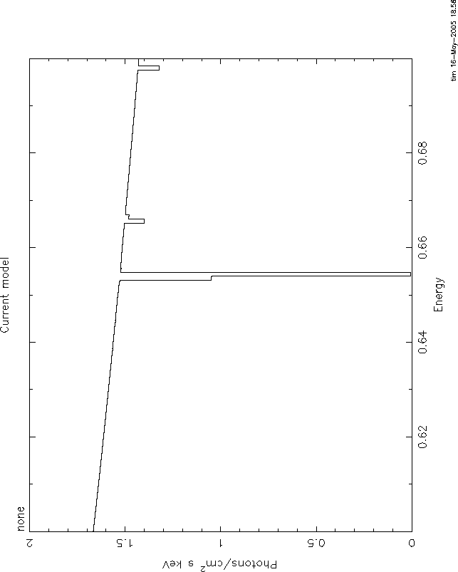
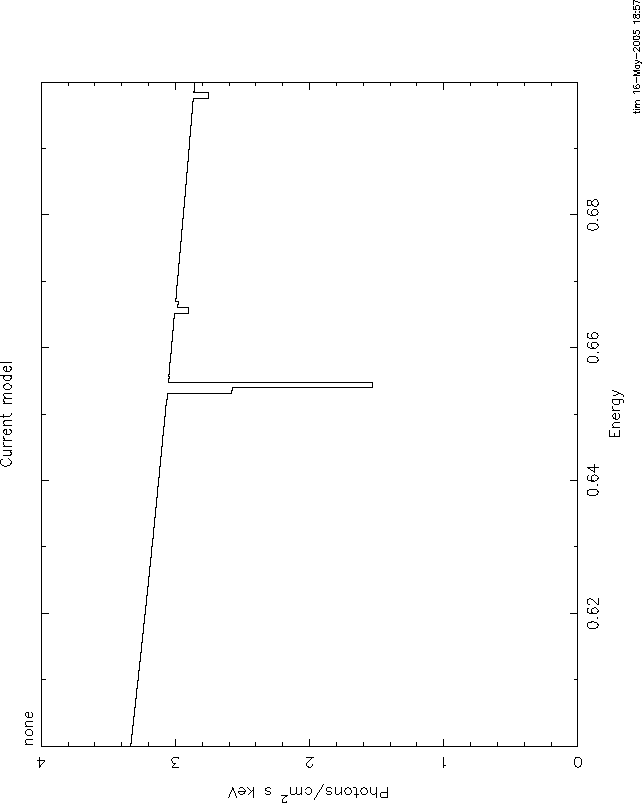
Here again, the problem is that even the pure oxygen mtable has the
transmittivity of the 'zero abundance' model, ![]() , which really has pure
H and He and therefore has unit transmittivity. The line never can go
black. The only model which is nearly correct is 3, but here again you
have the problem of multiple counting of the H and He opacity. But at
this high ionization parameter that is negligible. Anyway, I hope you
understand the problem.
, which really has pure
H and He and therefore has unit transmittivity. The line never can go
black. The only model which is nearly correct is 3, but here again you
have the problem of multiple counting of the H and He opacity. But at
this high ionization parameter that is negligible. Anyway, I hope you
understand the problem.
It is straightforward to use xstar2xspec to calculate grids without variable abundances. THEN you can use mtables, and there should be none of these problems.
Question:
I have made some comparisons between vturb=0 models and those with vturb=100. I find that vturb=0 gave very different results (much less absorption) to the vturb=100 grid18 etable. I hadn't expected to see the large difference with a change from vturb=100 to vturb=0. Is this expected behaviour?
Answer:
vturb can make a significant difference in the results of xstar modeling of absorption spectra, and the reason is at least partially due to numerics. In calculating the energy dependent opacity Xstar simply evaluates the profile function for the line at each grid energy. So if the line width is less than, or comparable to, the xstar grid spacing, then maximum depth of a given absorption line in the mtable may be very different from the true depth at line center. Obviously this problem is more severe for small vturb, i.e. narrow lines. The total line equivalent width does not depend on vturb, but the numerics do not reflect that unless the line is broader than the grid resolution. And the limiting resolution is the internal xstar grid spacing, which corresponds to 420 km/s, since this is what is used in constructing the table. This is another flaw in the use of tables for fitting to spectra.
_________________________________________________________________________________
There is now subroutine which calculates xstar warm absorber (called 'warmabs') and warm emitter (called 'photemis') spectra and which can be called as an xspec `analytic' model. This calculates absorption spectra `on the fly', and so will evaluate the profile function on whatever grid you use in xspec. So you can choose to resolve all the lines if you want, using the 'dummyrsp' command with a very large number of bins. It is available on the xstar web site, look for the link under `XSTAR news'. It also does not suffer from the problems discussed previously about the approximations inherent in variable abundance. It calculates the opacity directly from a stored library of level populations calculated for a generic power law grid.
One drawback of this routine is that it brute-force calculates Voigt profiles and opacity for all the lines and bound-free continua which are above a certain threshold in strength, and so it is time-consuming. Currently calls to this routine can take up to 30 seconds on a slow or busy machine. It will be much faster on a faster machine, or if there are few elements with non-zero abundances, or if only a narrow spectral range is of interest, or if the ionization parameter is frozen.
Another drawback to this routine is that the current version assumes constant ionization throughout a slab of given ionization parameter and column. Real slabs will have lower mean ionization in the deeper, shielded regions, and this lower ionization material will absorb more efficiently. This means that the current warmabs assumption results in an underestimate of the opacity, particularly at low energies, for slabs with large column. This will be remedied in future versions of this routine.
_________________________________________________________________________________
Yet another issue which deserves mention is that of interpolation and grid spacing in the interpolated parameters as implemented by xspec. Many of the available xstar grids were calculated with models spaced 1 decade apart in column. This has the potential to lead to inaccuracies in the model spectrum calculated by xspec, since it will interpolate between grid points. Sparsely gridded models may miss important details. Grids 19b and 19c provide an example.
_________________________________________________________________________________
Question:
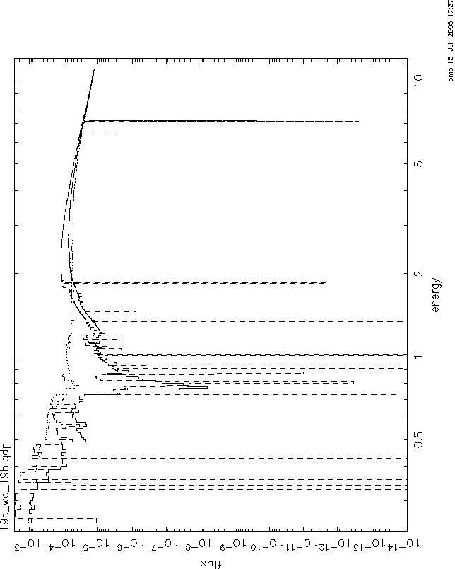
I have compared the grids with the warmabs analytical model. These are in
firgure 5. 19c is the solid line, warmabs is the dashed line, and 19b
is the dotted line. The model here is the same model that I used to fit
the data using 19c (ie, it has 1.4e20 of wabs also). I hope you can get
some info from this. The parameters used for these models were: log![]() =1.27,
N=5.89e22.
=1.27,
N=5.89e22.
Answer:
OK, so what I see from your plot comparing the models is that:
1) grid19b and grid19c give qualitatively different results near the best fit parameter values in the strength of the absorption near the K edge of oxygen. This seems to me to be clear evidence for the errors introduced by interpolation in a sparsely gridded table in column, as I suggested.
2) grid19c and warmabs agree well at energies above .8 keV, except for the lines. This seems to me to be a comforting check on the validity of warmabs.
3) there is disagreement in the strength of the absorption below 0.8 keV.
We decided that the assumption of a constant ionization slab made in
warmabs would tend to underestimate the absorption, since the ionization
balance would be lower in the shielded parts of a real slab, hence more
absorption. This is the sense of the disagreement, and so seems to make
sense. Of course, there is still some interpolation involved in the use
of grid19c, since your best fit values for N and ![]() are not precisely on
the grid values. I have compared warmabs and grid19c for the nearest grid
values, and the effect of interpolation does not appear to change the
sense of the disagreement. So this is a strong argument for fixing up
warmabs so that it does not make the uniform slab assumption.
are not precisely on
the grid values. I have compared warmabs and grid19c for the nearest grid
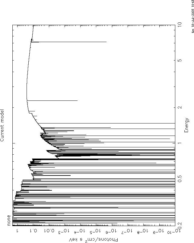
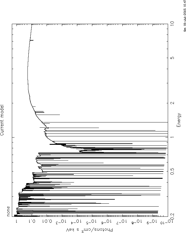
values, and the effect of interpolation does not appear to change the
sense of the disagreement. So this is a strong argument for fixing up
warmabs so that it does not make the uniform slab assumption.
4) There is also disagreement between grid19c and warmabs about the strength of the lines. I think this is due to the effect of energy binning: Your energy grid must be rather coarse, i.e.R=E/Delta(E) 100. If you make the same plot with a grid resolution of R=10000, things look better. I attach these plots: figure 6=warmabs, figure 7=grid19c. But there is still disagreement, and this I think is because the grid19c results have the intrinsic xstar internal resolution, which is much less than 10000, and so information is lost about the line profiles, while warmabs calculates the lines specifically for the resolution requested, and so should be more accurate.