Next: Speeding Things Up Up: Running XSTAR2XSPEC Previous: Important Notes on Mtables Contents
The problem with creating a flexible tool for modelling emission and absorption is that there have several free parameters affecting real spectra, including: source luminosity, distance, reprocessor column density, ionization parameter, and geometry. By geometry we mean covering fraction around the source, which affects emission, and covering fraction across our line of sight to the source, which affects absorption. With the xstar2xspec tables you should be able to model a wide range of choices for this, but there is not a unique one-to-one mapping between the values of these physical parameters and the values used in running xstar and constructing the tables.
The free parameters which can be varied when running xstar2xspec include the abundances, column density, gas density, and ionization parameter. These all have a straightforward intepretation as physical parameters. The emitter normalization and geometry are not uniquely determined, owing to the ambiguity between source luminosity and distance.
It is helpful here to be very specific, at the risk of being repetitive.
The procedure followed by xstar2xspec in making tables is: (i) Generate
a sequence of command line calls to xstar (this is done by the tool xstinitable);
(ii) step through the calls to xstar; (iii) for each one calculate the appropriate
xstar model; (iv) and then take the spectrum output of the model (the file xout_spect1.fits) and
convert it to the right units and append it to the fits table (xout_aout.fits, xout_ain.fits,
or xout_mtable.fits). The last step (iv) is done by the tool xstar2table. The conversion
is as follows: xspec wants a binned spectrum in units model counts/bin for atables.
If this is denoted ![]() , and the luminosity used in calculating the xstar grid is
, and the luminosity used in calculating the xstar grid is
![]() then
then
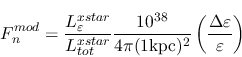
which can be rewritten:
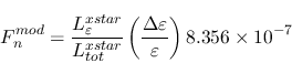
and
![]() is the fractional energy bin size.
is the fractional energy bin size.
The meaning of this quantity and the normalization can be better understood if we consider how
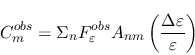
xspec works in more detail. Xspec calculates the model count rates per bin by multiplying the
![]() vector with the response matrix
vector with the response matrix ![]() and multiplying by a normalization factor
and multiplying by a normalization factor ![]() :
:
The observed count rate ![]() is calculated from the physical flux recieved by the
satellite
is calculated from the physical flux recieved by the
satellite
![]() :
:
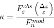
Then it's easy to see that
![]() if the shape of the model fits the observations and
if the shape of the model fits the observations and

or
Now, if the astronomical X-ray source actually resembles the physical scenario assumed by xstar, i.e. if it
consists of a shell of photoionized material surrounding
a point source of continuum with covering fraction ![]() then
then
![]() , where
, where
![]() is the actual specific luminosity emitted by the shell, and
is the actual specific luminosity emitted by the shell, and ![]() is the distance
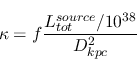
to the source. Then
is the distance
to the source. Then
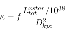
And, if we have gotten the model exactly right and
![]() (which implies that
(which implies that
![]() ) then
) then
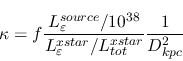
If, on the other hand, the shape of the emitted spectrum is right but the luminosity of the astrophyscial source is
different from the luminosity used in calculating the xstar model then
![]() and
and
which can be inverted to find the things on the right hand side if you have a fitted value for ![]() .
.
So, for example, if your atable model fits to the data with a normalization=1, let's say,
and you used luminosity=1 in creating the table, then this would
imply that your data was consistent with a full shell illuminated
by a luminosity of 10![]() erg/s at a distance of 1 kpc,
or it also could be a shell illuminated by a luminosity of 10
erg/s at a distance of 1 kpc,
or it also could be a shell illuminated by a luminosity of 10![]() erg/s
at a distance of 1000 kpc.
erg/s
at a distance of 1000 kpc.
For another example, let's say you know the distance to the source
is 1 kpc and the luminosity is 10![]() , but the best fit has an emitter
normalization of 0.1. This would suggest (to me) that rather than
a full sphere, the emitter only subtends 10
, but the best fit has an emitter
normalization of 0.1. This would suggest (to me) that rather than
a full sphere, the emitter only subtends 10![]() of the solid angle around the
source.
of the solid angle around the
source.
Obviously, the column density of the emitter is important also. If you
don't know the column density, then a shell of column density 10![]() cm
cm![]() illuminated by a 10
illuminated by a 10![]() erg s
erg s![]() source will probably have very
similar emitted X-ray spectrum to a shell of column density 10
source will probably have very
similar emitted X-ray spectrum to a shell of column density 10![]() illuminated by a
10
illuminated by a
10![]() erg s
erg s![]() source. If there are absorption features in the
spectrum, then they may constrain the column density.
source. If there are absorption features in the
spectrum, then they may constrain the column density.