

Data Simulation and Analysis Threads
Fit OM + EPIC Spectrum with Sherpa
Data from OM and EPIC (and/or RGS) can be analyzed in Sherpa using the usual methods. For this example, the data set is from the Lockman Hole (ObsID 0123700101) observation for which we reprocessed EPIC and OM data. We will use the MOS1 spectrum with headers that have already been edited so Sherpa will automatically load the response files. (The OM PHA files have headers that are automatically set to the canned response files). One thing to note here is that the canned responses are *.rsp files, not arfs and rmfs, which Sherpa needs. Luckily, it is straightforward to transform them into the needed format with ftools.
   tar xvfz om_effarea_v2.0.tgz
   ftools
   ftrsp2rmfarf om_effarea_uvw1_v2.0.rsp om_effarea_uvw1_v2.0.rmf om_effarea_uvw1_v2.0.arf
   ftrsp2rmfarf om_effarea_uvw2_v2.0.rsp om_effarea_uvw2_v2.0.rmf om_effarea_uvw2_v2.0.arf
   ftrsp2rmfarf om_effarea_u_v2.0.rsp om_effarea_u_v2.0.rmf om_effarea_u_v2.0.arf
   ftrsp2rmfarf om_effarea_v_v2.0.rsp om_effarea_v_v2.0.rmf om_effarea_v_v2.0.arf
With the OM response files ready to go, fitting them is the same as fitting any data set. For our example, the χ2 statistic is fine, so we will rebin the data. Remember to use a window in which SAS has not been initialized. We will load in all the data, do a very naïve fit, and plot the result.
ciao
sherpa
load_pha(1, "mos1_pi.fits") # read in the EPIC source spectrum and its associated files
ignore(":0.5, 3.0:") # set some reasonable limits
group_counts(20) # rebin the data to a minimum of 20 counts/bin
subtract() # subtract the background
load_pha(2, "om_src.pi", use_errors=True) # read in the OM data and their associated files
load_rmf(2, "om_effarea_uvw2_v2.0.rmf")
load_rmf(3, "om_effarea_uvw1_v2.0.rmf")
load_rmf(4, "om_effarea_u_v2.0.rmf")
load_rmf(5, "om_effarea_v_v2.0.rmf")
load_arf(2, "om_effarea_uvw2_v2.0.arf")
load_arf(3, "om_effarea_uvw1_v2.0.arf")
load_arf(4, "om_effarea_u_v2.0.arf")
load_arf(5, "om_effarea_v_v2.0.arf")
set_source(1, xspowerlaw.p1) # define the model
set_source(2, xspowerlaw.p1)
set_source(3, xspowerlaw.p1)
set_source(4, xspowerlaw.p1)
set_source(5, xspowerlaw.p1)
fit() # automatically fit all loaded data sets simultaneously
set_xlog() # use a log-log plot
set_ylog()
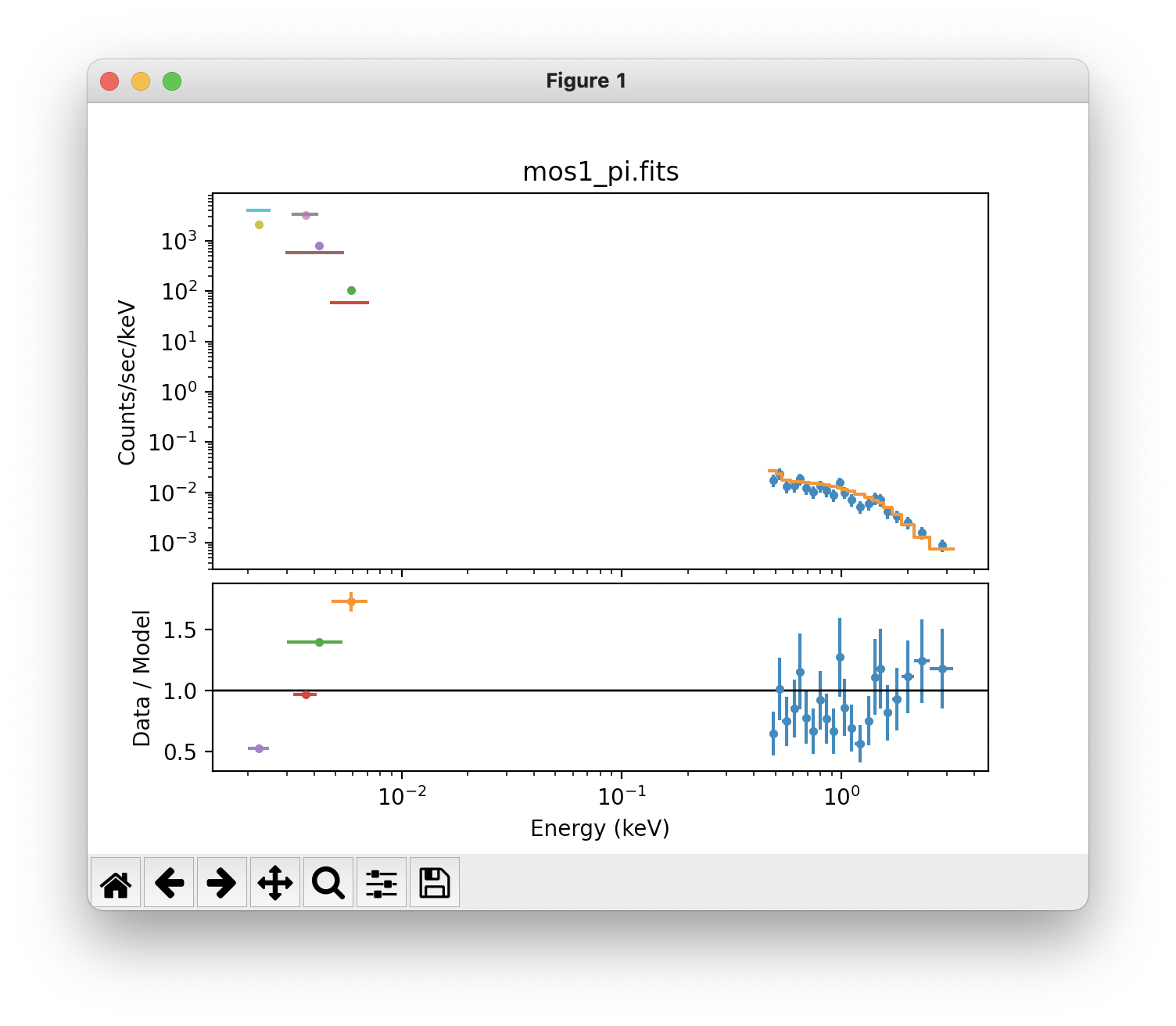
plot_fit_ratio()
plot_fit_ratio(2, overplot=True)
plot_fit_ratio(3, overplot=True)
plot_fit_ratio(4, overplot=True)
plot_fit_ratio(5, overplot=True)
The fit is shown in Figure 1.
|
More information about Sherpa, including models and walk-throughs, can be found here.
If you have any questions concerning XMM-Newton send e-mail to xmmhelp@lists.nasa.gov