Suzaku has five light-weight thin-foil X-Ray Telescopes (XRTs). The XRTs have been developed jointly by NASA/GSFC, Nagoya University, Tokyo Metropolitan University, and ISAS/JAXA. These are grazing-incidence reflective optics consisting of compactly nested, thin conical elements. Because of the reflectors' small thickness, they permit high density nesting and thus provide large collecting efficiency with a moderate imaging capability in the energy range of 0.2-12keV, all accomplished in telescope units under 20kg each.
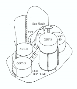
Four XRTs on-board Suzaku are used for the XIS (XRT-I), and the remaining XRT is for the XRS (XRT-S). XRT-S is no longer functional. The XRTs are arranged on the Extensible Optical Bench (EOB) on the spacecraft in the manner shown in Fig. 6.1. The external dimensions of the 4 XRT-Is are the same (see Table 6.1, which also includes a comparison with the ASCA telescopes).
The angular resolutions of the XRTs range from ![]() to
to ![]() ,
expressed in terms of half-power diameter, which is the diameter
within which half of the focused X-rays are enclosed. The angular
resolution does not significantly depend on the energy of the incident
X-rays in the energy range of Suzaku, 0.2-12keV. The effective areas
are typically 440cm
,
expressed in terms of half-power diameter, which is the diameter
within which half of the focused X-rays are enclosed. The angular
resolution does not significantly depend on the energy of the incident
X-rays in the energy range of Suzaku, 0.2-12keV. The effective areas
are typically 440cm![]() at 1.5keV and 250cm
at 1.5keV and 250cm![]() at
8keV. The focal length of the XRT-I is 4.75m. Actual focal lengths
of the individual XRT quadrants deviate from the design values by a
few cm. The optical axes of the quadrants of each XRT are aligned to
within 2
at
8keV. The focal length of the XRT-I is 4.75m. Actual focal lengths
of the individual XRT quadrants deviate from the design values by a
few cm. The optical axes of the quadrants of each XRT are aligned to
within 2![]() from the mechanical axis. The field of view for
the XRT-Is is about 17
from the mechanical axis. The field of view for
the XRT-Is is about 17![]() at 1.5keV and 13
at 1.5keV and 13![]() at
8keV (see also Table 3.1).
at
8keV (see also Table 3.1).
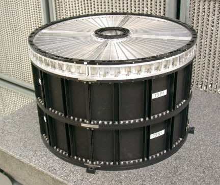
The Suzaku X-Ray Telescopes (XRTs) consist of closely nested thin-foil
reflectors, reflecting X-ray at small grazing angles. An XRT is a
cylindrical structure, having the following layered components: 1. a
thermal shield at the entrance aperture to help maintain a uniform
temperature, 2. a pre-collimator mounted on metal rings for stray
light elimination, 3. a primary stage for the first X-ray reflection,
4. a secondary stage for the second X-ray reflection, 5. a base ring
for structural integrity and interfacing with the EOB of the
spacecraft. All these components, except the base rings, are
constructed in 90
![]() segments. Four of these quadrants
are coupled together by interconnect-couplers and also by the top and
base rings (Fig. 6.2). The telescope housings are made
of aluminum for an optimal strength to mass ratio. Each reflector
consists of a substrate also made of aluminum and an epoxy layer that
couples the reflecting gold surface to the substrate.
segments. Four of these quadrants
are coupled together by interconnect-couplers and also by the top and
base rings (Fig. 6.2). The telescope housings are made
of aluminum for an optimal strength to mass ratio. Each reflector
consists of a substrate also made of aluminum and an epoxy layer that
couples the reflecting gold surface to the substrate.
Including the alignment bars, collimating pieces, screws and washers,
couplers, retaining plates, housing panels and rings, each XRT-I
consists of over 4112 mechanically separated parts. In total, nearly
7000 qualified reflectors were used and over 1 millioncm![]() of gold surface was coated.
of gold surface was coated.
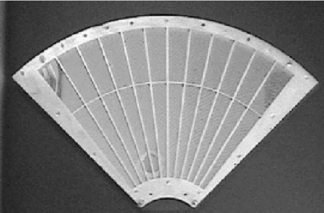
In shape, each reflector is a 90
![]() segment of a
section of a cone. The cone angle is designed to be the angle of
on-axis incidence for the primary stage and 3 times that for the
secondary stage. They are 101.6mm in slant length, with radii
extending approximately from 60mm at the inner part to 200mm at
the outer part. The reflectors are nominally 178
segment of a
section of a cone. The cone angle is designed to be the angle of
on-axis incidence for the primary stage and 3 times that for the
secondary stage. They are 101.6mm in slant length, with radii
extending approximately from 60mm at the inner part to 200mm at
the outer part. The reflectors are nominally 178
![]() m in
thickness. All reflectors are positioned with grooved alignment bars,
which hold the foils at their circular edges. There are 13 alignment
bars at the face of each quadrant, separated by
m in
thickness. All reflectors are positioned with grooved alignment bars,
which hold the foils at their circular edges. There are 13 alignment
bars at the face of each quadrant, separated by
![]() 6.4
6.4
![]() .
.
To properly reflect and focus X-ray at grazing incidence, the
precision of the reflector figure and the smoothness of the reflector
surface are important aspects. Since polishing of thin reflectors is
both impractical and expensive, reflectors in Suzaku XRTs acquire their
surface smoothness by a replication technique and their shape by
thermo-forming of aluminum. In the replication method, metallic gold
is deposited on an extrusion glass mandrel (``replication mandrel''),
the surface of which has sub-nanometer smoothness over a wide spatial
frequency, and the substrate is subsequently bonded with the metallic
film with a layer of epoxy. After the epoxy is hardened, the
substrate-epoxy-gold film composite can be removed from the glass
mandrel and the replica acquires the smoothness of the glass. The
replica typically has
![]() 0.5nm rms roughness at mm or
smaller spatial scales, which is sufficient for excellent reflectivity
at incident angles less than the critical angle. The Suzaku XRTs are
designed with on-axis reflection at less than the critical angle,
which is approximately inversely proportional to X-ray energy.
0.5nm rms roughness at mm or
smaller spatial scales, which is sufficient for excellent reflectivity
at incident angles less than the critical angle. The Suzaku XRTs are
designed with on-axis reflection at less than the critical angle,
which is approximately inversely proportional to X-ray energy.
In the thermo-forming of the substrate, pre-cut, mechanically rolled
aluminum foils are pressed onto a precisely shaped ``forming
mandrel'', which is not the same as the replication mandrel. The
combination is then heated until the aluminum softens. The aluminum
foils acquire the shape of the properly shaped mandrel after cooling
and release of pressure. In the Suzaku XRTs, the conical approximation
of the Wolter-I type geometry is used. This approximation
fundamentally limits the angular resolution achievable. More
significantly, the combination of the shape error in the replication
mandrels and the imperfection in the thermo-forming process (to about
4![]() m in the low frequency components of the shape error in the
axial direction) limits the angular resolution to about 1
m in the low frequency components of the shape error in the
axial direction) limits the angular resolution to about 1![]() .
.
The pre-collimator, which blocks stray light that otherwise would
enter the detector at a larger angle than intended, consists of
concentrically nested aluminum foils, similar to those of the
reflector substrates. They are shorter, 22mm in length, and thinner,
120![]() m in thickness. They are positioned in a fashion similar to
that of the reflectors, by 13 grooved aluminum plates at each circular
edge of the pieces. They are installed on top of their respective
primary reflectors along the axial direction. Due to their smaller
thickness, they do not significantly reduce the entrance aperture in
that direction more than the reflectors already do. Pre-collimator
foils do not have reflective surfaces (neither front nor back). The
relevant dimensions are listed in Table 6.2.
m in thickness. They are positioned in a fashion similar to
that of the reflectors, by 13 grooved aluminum plates at each circular
edge of the pieces. They are installed on top of their respective
primary reflectors along the axial direction. Due to their smaller
thickness, they do not significantly reduce the entrance aperture in
that direction more than the reflectors already do. Pre-collimator
foils do not have reflective surfaces (neither front nor back). The
relevant dimensions are listed in Table 6.2.
The Suzaku XRTs are designed to function in a thermal environment of
20
![]() 7.5
7.5
![]() C. The reflectors, due to
their composite nature and thus their mismatch in coefficients of
thermal expansion, suffer from thermal distortion that degrades the
angular resolution of the telescopes for temperatures outside this
range. Thermal gradients also distort the telescope on a larger
scale. Even though sun shields and other heating elements on the
spacecraft help in maintaining a reasonable thermal environment,
thermal shields are integrated on top of the pre-collimator stage to
provide the needed thermal control.
C. The reflectors, due to
their composite nature and thus their mismatch in coefficients of
thermal expansion, suffer from thermal distortion that degrades the
angular resolution of the telescopes for temperatures outside this
range. Thermal gradients also distort the telescope on a larger
scale. Even though sun shields and other heating elements on the
spacecraft help in maintaining a reasonable thermal environment,
thermal shields are integrated on top of the pre-collimator stage to
provide the needed thermal control.
In this section we describe the in-flight performance and calibration of the Suzaku XRTs. There are no data to verify the in-flight performance of the XRT-S, therefore we hereafter concentrate on the four XRT-I modules (XRT-I0 through I3) which focus incident X-rays on the XIS detectors. Several updates of the XRT-related calibration were made in July 2008.
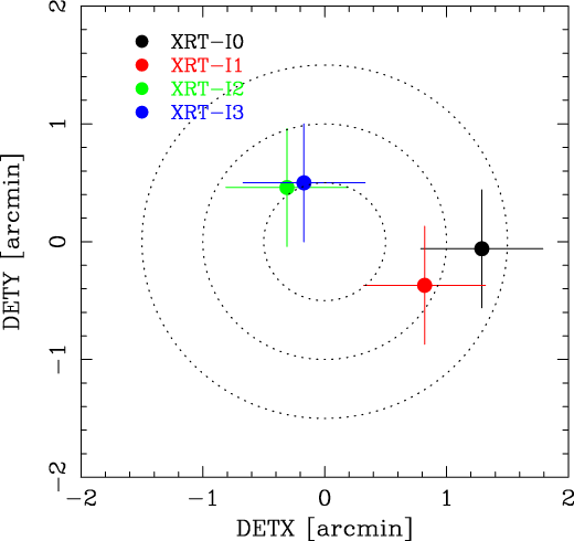
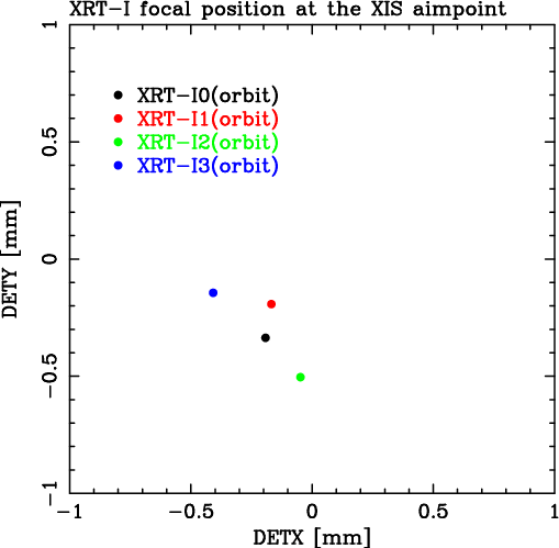
A point-like source, MCG![]() 6-30-15, was observed at the XIS aim point
during 2005 August 17-18. Fig. 6.4 shows the focal position
of the XRT-Is, that the source is found at on the XISs, when the
satellite points at it using the XIS aim point. The focal positions
are located close to the detector center with a deviation of 0.3mm
from each other. This implies that the fields of view of the XISs
coincide to within
6-30-15, was observed at the XIS aim point
during 2005 August 17-18. Fig. 6.4 shows the focal position
of the XRT-Is, that the source is found at on the XISs, when the
satellite points at it using the XIS aim point. The focal positions
are located close to the detector center with a deviation of 0.3mm
from each other. This implies that the fields of view of the XISs
coincide to within ![]() .
.
|
The maximum transmission of each telescope module is achieved when a
target star is observed along the optical axis. The optical axes of
the four XRT-I modules are, however, expected to scatter in an angular
range of ![]() 1
1![]() . Accordingly, we have to define the axis to be
used for real observations that provides a reasonable compromise among
the four optical axes. We hereafter refer to this axis as the
observation axis.
. Accordingly, we have to define the axis to be
used for real observations that provides a reasonable compromise among
the four optical axes. We hereafter refer to this axis as the
observation axis.
In order to determine the observation axis, we have first searched for the optical axis of each XRT-I module by observing the Crab nebula at various off-axis angles. The observations of the Crab nebula were carried out in 2005 and 2006. Hereafter all the off-axis angles are expressed in the detector coordinate system DETX/DETY (see ftp://heasarc.gsfc.nasa.gov/suzaku/doc/xis/suzakumemo-2006-39.pdf.
By fitting a model comprising of a Gaussian plus a constant to the count rate data as a function of the off-axis angle, we have determined the optical axis of each XRT-I module. The result is shown in Fig. 6.5.
|
Since the optical axes moderately scatter around the origin, we have
decided to adopt it as the default observation axis for XIS-oriented
observations. Hereafter we refer to this axis as the XIS-default
orientation, or equivalently, the XIS-default position. The optical
axis of the XRT-I0 shows the largest deviation of ![]() from
the XIS-default position. Nevertheless, the efficiency of the XRT-I0
at the XIS-default position is more than 97%, even at 8-10keV, the
highest energy band (see Fig. 6.10). The optical axis of
the HXD PIN detector, on the other hand, deviates from this default by
from
the XIS-default position. Nevertheless, the efficiency of the XRT-I0
at the XIS-default position is more than 97%, even at 8-10keV, the
highest energy band (see Fig. 6.10). The optical axis of
the HXD PIN detector, on the other hand, deviates from this default by
![]() 5
5![]() in the negative DETX direction (see for example, the
instrument paper at ftp://heasarc.gsfc.nasa.gov/suzaku/doc/hxd/suzakumemo-2006-37.pdf).
Because of this, the observation efficiency of the HXD PIN at the
XIS-default orientation is reduced to
in the negative DETX direction (see for example, the
instrument paper at ftp://heasarc.gsfc.nasa.gov/suzaku/doc/hxd/suzakumemo-2006-37.pdf).
Because of this, the observation efficiency of the HXD PIN at the
XIS-default orientation is reduced to ![]() 93% of the on-axis value.
We thus provide another default pointing position, the HXD-default
position, for HXD-oriented observations, at
93% of the on-axis value.
We thus provide another default pointing position, the HXD-default
position, for HXD-oriented observations, at ![]() in
DETX/DETY coordinates. At the HXD-default position, the efficiency of
the HXD PIN is nearly 100%, whereas that of the XIS is
in
DETX/DETY coordinates. At the HXD-default position, the efficiency of
the HXD PIN is nearly 100%, whereas that of the XIS is ![]() 88% on
average.
88% on
average.
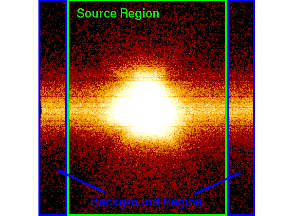
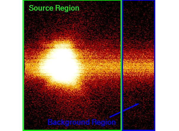
In-flight calibration of the effective area has been carried out with version 2.1 processed data of the Crab nebula both at the XIS- and HXD-default positions. The observations were carried out in 2005 September 15-16. The data were taken in the normal mode with the 0.1s burst option in which the CCD is exposed during 0.1s out of the full-frame read-out time of 8s, in order to avoid the event pile-up and the telemetry saturation. The exposure time of 0.1s is, however, comparable to the frame transfer time of 0.025s. As a matter of fact, the Crab image is elongated in the frame-transfer direction due to so-called the out-of-time events, as shown in Fig. 6.6.
|
Accordingly, the background-integration regions with a size of 126 by
1024 pixels are taken at the left and right ends of the chip for the
XIS-default position, perpendicularly to the frame-transfer direction,
as shown in the left panel of Fig. 6.6. For the
observation at the HXD-default position, the image center is shifted
from the XIS-default position in the direction perpendicular to the
frame-transfer direction for XIS0 and XIS3. Hence we can adopt the
same background-integration regions as those of the XIS-default
position for these two XIS modules. For XIS1 and XIS2, on the other
hand, the image shift occurs in the frame-transfer direction, as shown
in the right panel of Fig. 6.6. We thus take a
single background-integration region with a size of 252 by 1024 pixels
at the far side from the Crab image for the HXD-default position of
these two detectors. As a result, the remaining source-integration
region has a size of 768 by 1024 pixels, or
![]() for
all the cases, which is wide enough to collect all the photons from
the Crab nebula.
for
all the cases, which is wide enough to collect all the photons from
the Crab nebula.
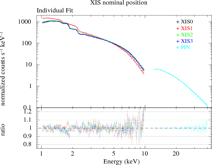
After subtracting the background, taking into account the sizes of the regions, we have fitted the spectra taken with the four XIS modules with a model composed of a power law undergoing photoelectric absorption using xspec Version 11.2. For the photoelectric absorption, we have adopted the model phabs with the cosmic metal abundances of Anders & Grevesse (1989, Geochim. Cosmochim. Acta, 53, 197). First, we let all parameters vary independently for all the XIS modules. The results are summarized for the XIS/HXD nominal positions separately in Table 6.3 and are shown in Fig. 6.7.
| Sensor ID | Photon Index | Normalization | Flux | ||
| XIS-default position | |||||
| XIS0 | 0.311 |
2.077 |
9.38
|
2.086 | 1.02 (89) |
| XIS1 | 0.294 |
2.085 |
9.73
|
2.141 | 1.59 (89) |
| XIS2 | 0.282 |
2.065 |
9.29
|
2.134 | 1.34 (89) |
| XIS3 | 0.304 |
2.082 |
9.33
|
2.062 | 1.34 (89) |
| PIN | 0.3 (fix) | 2.101 |
11.41 |
2.464 | 0.74 (72) |
| HXD-default position | |||||
| XIS0 | 0.304 |
2.079 |
9.13
|
2.025 | 1.28 (89) |
| XIS1 | 0.295 |
2.111 |
9.59
|
2.030 | 0.86 (89) |
| XIS2 | 0.282 |
2.070 |
9.54
|
2.151 | 1.22 (89) |
| XIS3 | 0.301
|
2.085 |
9.29 |
2.043 | 1.19 (89) |
| PIN | 0.3 (fix) | 2.090 |
10.93 |
2.400 | 0.82 (72) |
|
For the fit, we have adopted the ARFs and RMFs generated using CALDB
2008-07-09. These ARFs are made for a point source, whereas the Crab
nebula is slightly extended (![]() 2
2![]() ). We thus have created ARFs by
utilizing the ray-tracing simulator (Misaki et al. 2005, Appl. Opt.,
44, 916) with a Chandra image as input, and have confirmed
that the difference of the effective area between these two sets of
ARFs is less than 1%. We have neglected the energy channels below
1keV, above 10keV, and in the 1.5-2.0keV band because of
insufficient calibration related to uncertainties of the nature and
amount of the contaminant on the OBF and to the Si edge structure (see
ftp://heasarc.gsfc.nasa.gov/suzaku/doc/hxd/suzakumemo-2006-35.pdf).
Data in the 1.5-2.0keV range are retrieved after the fit and shown
in Fig. 6.7.
). We thus have created ARFs by
utilizing the ray-tracing simulator (Misaki et al. 2005, Appl. Opt.,
44, 916) with a Chandra image as input, and have confirmed
that the difference of the effective area between these two sets of
ARFs is less than 1%. We have neglected the energy channels below
1keV, above 10keV, and in the 1.5-2.0keV band because of
insufficient calibration related to uncertainties of the nature and
amount of the contaminant on the OBF and to the Si edge structure (see
ftp://heasarc.gsfc.nasa.gov/suzaku/doc/hxd/suzakumemo-2006-35.pdf).
Data in the 1.5-2.0keV range are retrieved after the fit and shown
in Fig. 6.7.
Toor & Seward (1974, AJ, 79, 995) compiled the results from a number
of rocket and balloon measurements available at that time, and derived
the photon index and the normalization of the power law of the Crab
nebula to be ![]() and 9.7photons cm
and 9.7photons cm![]() s
s![]() keV
keV![]() at 1keV, respectively. Overlaying photoelectric
absorption with
at 1keV, respectively. Overlaying photoelectric
absorption with
![]() cm
cm![]() , we obtain the
flux to be
, we obtain the
flux to be
![]() erg cm
erg cm![]() s
s![]() in the
2-10keV band. The best-fit parameters of all the XIS modules at the
XIS- and HXD-default positions are close to these standard values.
in the
2-10keV band. The best-fit parameters of all the XIS modules at the
XIS- and HXD-default positions are close to these standard values.
Since the best-fit parameters of the four XIS modules are close to the standard values, we have attempted to constrain the photon index to be the same for all the detectors. The best-fit parameters are summarized in Table 6.4.
| Sensor ID | Photon Index | Normalization | Flux | ||
| XIS-default position | |||||
| XIS0 | 0.321 |
2.090 |
9.55 |
2.080 | 1.24 (432) |
| XIS1 | 0.298 |
9.79 |
2.14 | ||
| XIS2 | 0.302 |
9.72 |
2.13 | ||
| XIS3 | 0.311 |
9.43 |
2.06 | ||
| PIN | 0.3 (fix) | 11.06 |
2.42 | ||
| HXD-default position | |||||
| XIS0 | 0.307 |
2.086 |
9.19
|
2.019 | 1.13 (432) |
| XIS1 | 0.277 |
9.28 |
2.11 | ||
| XIS2 | 0.298 |
9.74 |
2.21 | ||
| XIS3 | 0.300 |
9.28 |
2.11 | ||
| PIN | 0.3 (fix) | 10.80 |
2.45 | ||
The hydrogen column density (0.28-0.32)
![]() cm
cm![]() and the photon index 2.09
and the photon index 2.09![]() 0.01 are consistent with the standard
values.
0.01 are consistent with the standard
values.
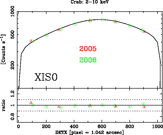
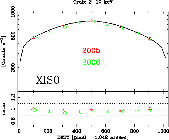
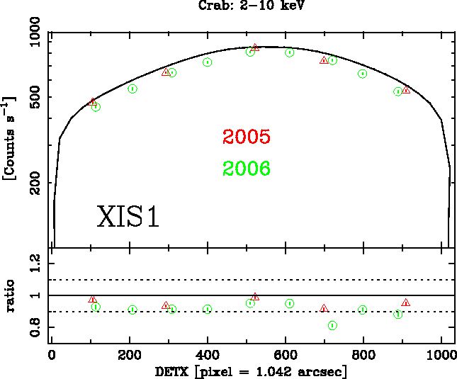
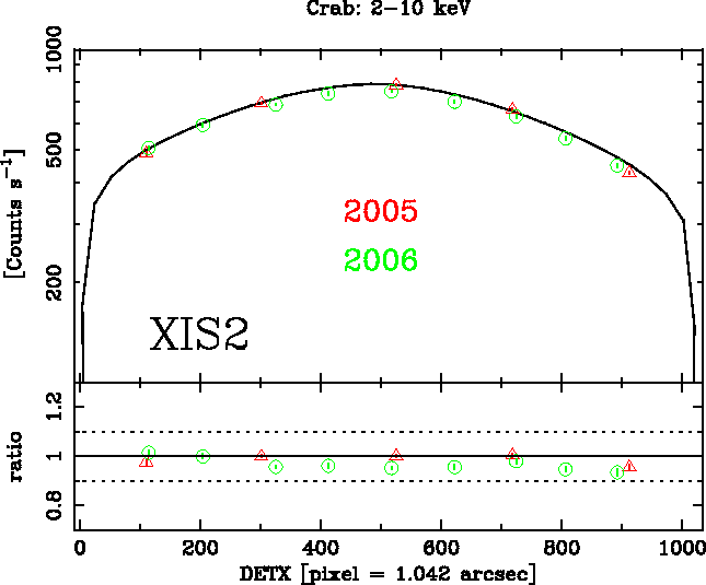
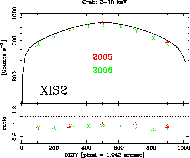
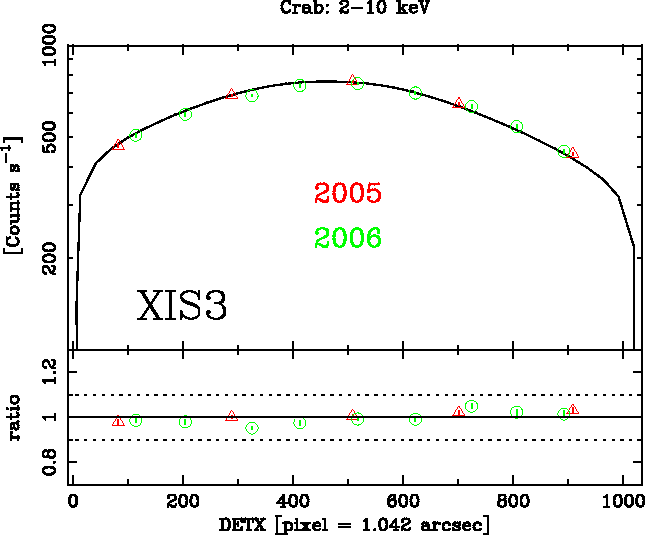
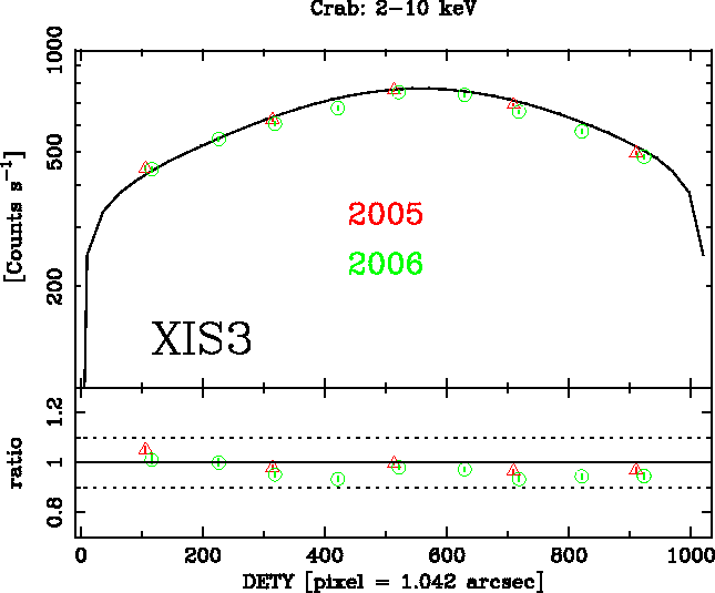
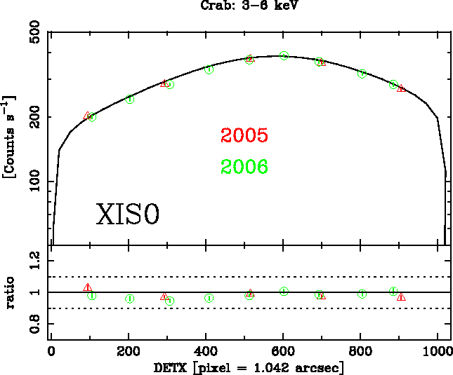
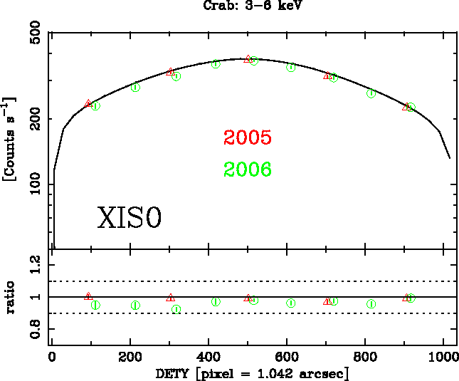
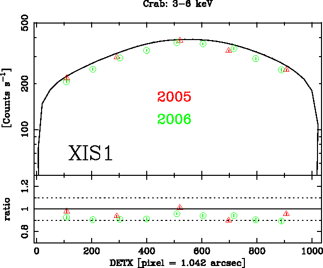
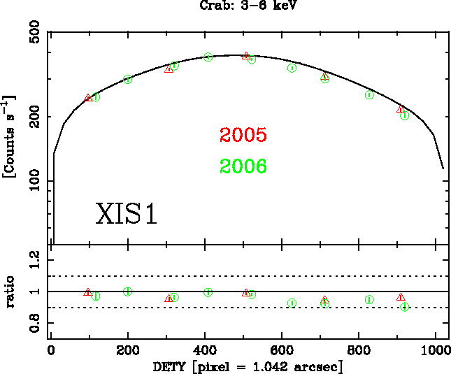
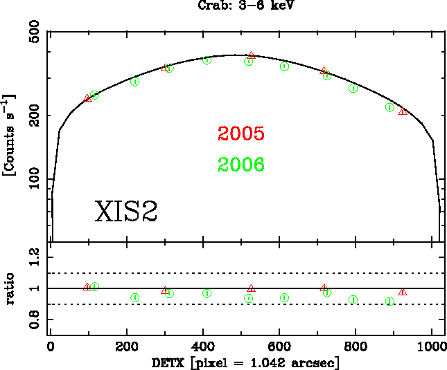
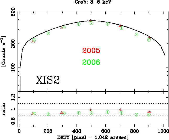
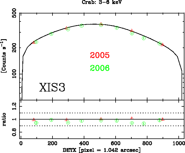
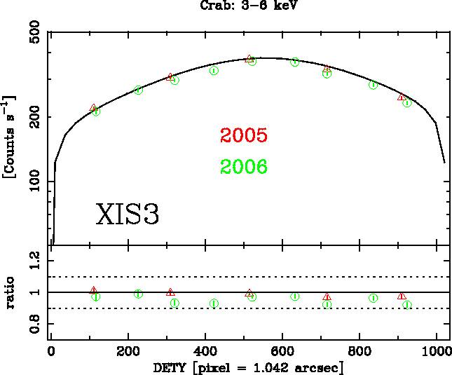
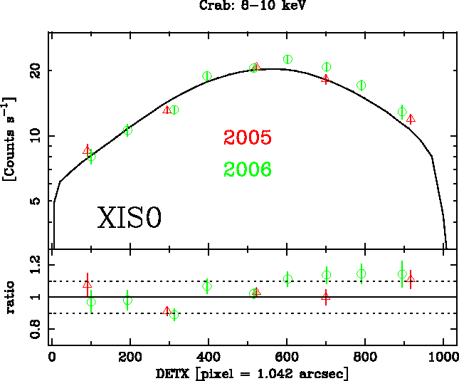
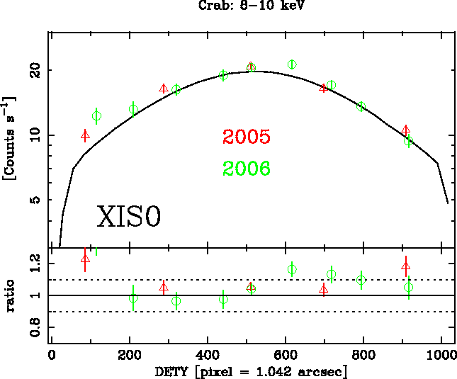
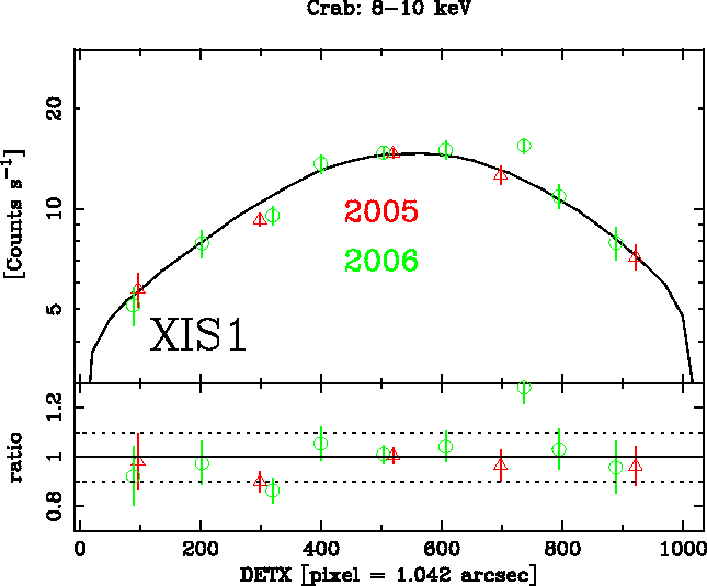
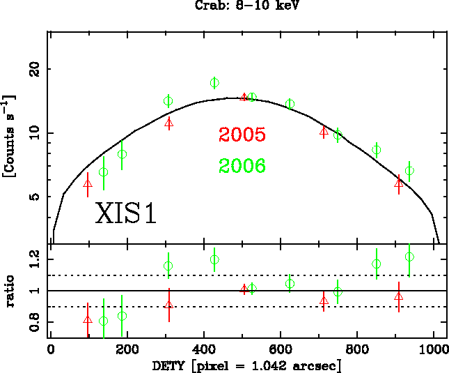
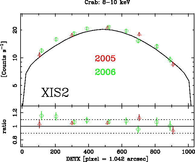
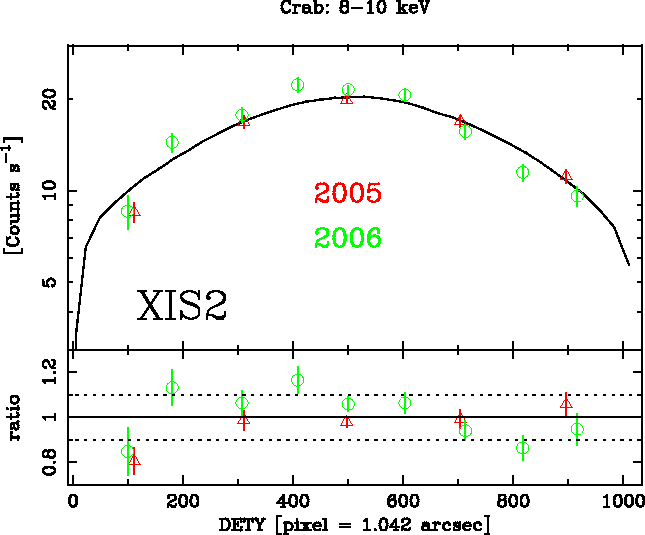
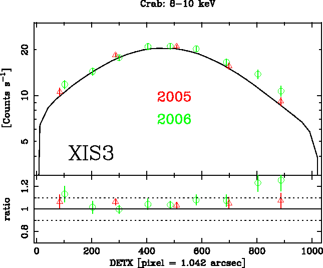
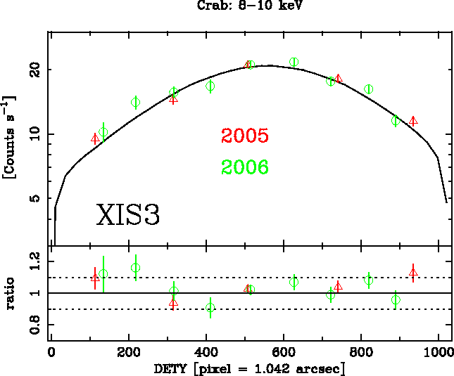
The vignetting curves calculated by the ray-tracing simulator are compared with the observed intensities of the Crab nebula at various off-axis angles in Figs. 6.8-6.10.
|
We have utilized the data of the Crab nebula taken during 2005 August
and 2006 August. In the figures, we have drawn the vignetting curves
for the energy bands 2-10keV, 3-6keV and 8-10keV. To obtain
this, we first assume the spectral parameters of the Crab nebula to be
a power law with
![]() cm
cm![]() , photon
index
, photon
index![]() 2.09, and normalization
2.09, and normalization![]() 9.845photons cm
9.845photons cm![]() s
s![]() keV
keV![]() at 1keV. These values are the averages of the four
detectors at the XIS-default position
(Table 6.4). We then calculate the count rate of the
Crab nebula on the entire CCD field of view in
at 1keV. These values are the averages of the four
detectors at the XIS-default position
(Table 6.4). We then calculate the count rate of the
Crab nebula on the entire CCD field of view in ![]() steps in both
the DETX and DETY directions using the ray-tracing simulator. Note
that the abrupt drop of the model curves at
steps in both
the DETX and DETY directions using the ray-tracing simulator. Note
that the abrupt drop of the model curves at ![]() 8
8![]() is due to the
source approaching the detector edge. On the other hand, the data
points provide the real count rates in the corresponding energy bands
within an aperture of
is due to the
source approaching the detector edge. On the other hand, the data
points provide the real count rates in the corresponding energy bands
within an aperture of ![]() by
by ![]() . Note that the aperture
adopted for the observed data can collect more than 99% of the
photons from the Crab nebula, and hence the difference of the
integration regions between the simulation and the observation does
not matter. Finally, we re-normalize both the simulated curves and the
data so that the count rate of the simulated curves at the origin
becomes equal to unity.
. Note that the aperture
adopted for the observed data can collect more than 99% of the
photons from the Crab nebula, and hence the difference of the
integration regions between the simulation and the observation does
not matter. Finally, we re-normalize both the simulated curves and the
data so that the count rate of the simulated curves at the origin
becomes equal to unity.
These figures roughly show that the effective area is calibrated
within ![]() 5% over the XIS field of view, except for the 8-10keV
band of XIS1. The excess of these XIS1 data points at the XIS-default
position has already been seen in Fig. 6.7 (see also
Table 6.3).
5% over the XIS field of view, except for the 8-10keV
band of XIS1. The excess of these XIS1 data points at the XIS-default
position has already been seen in Fig. 6.7 (see also
Table 6.3).
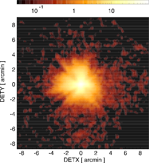
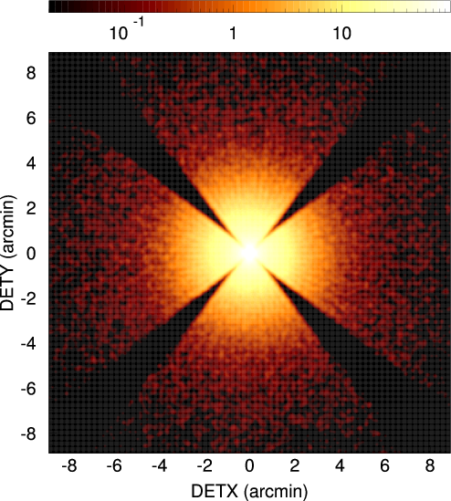
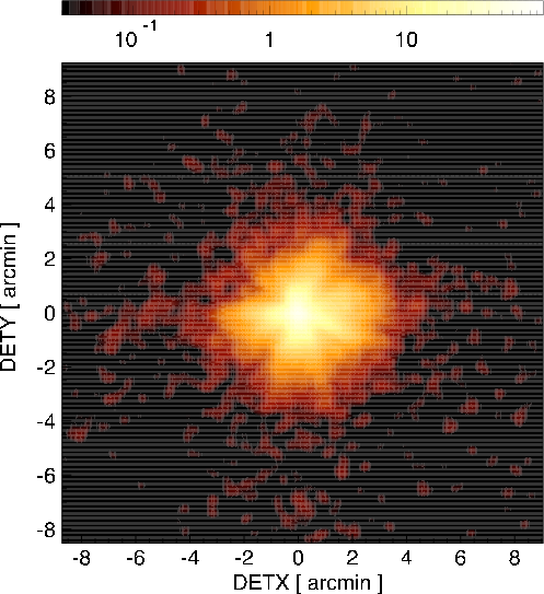
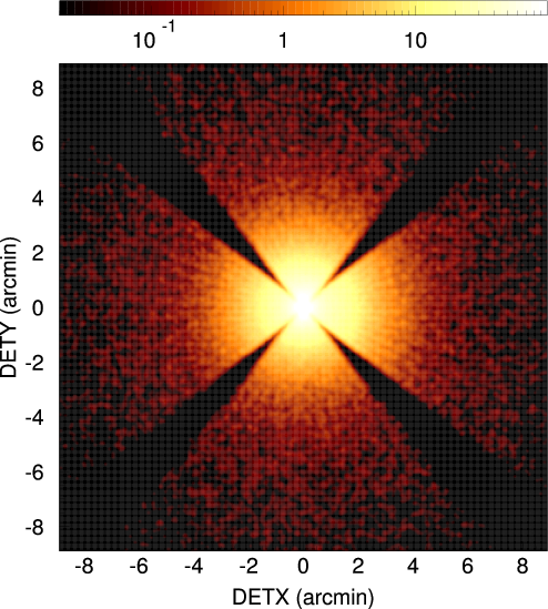
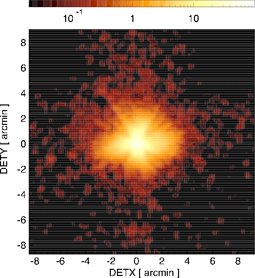
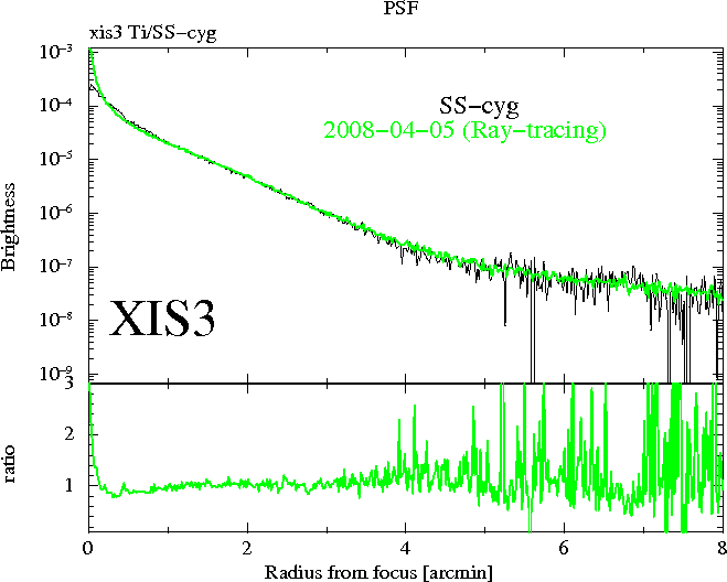
As shown in Serlemitsos et al. (2007), verification of the imaging
capability of the XRTs has been made with the data of SS Cyg in
quiescence taken on 2005 November 2 01:02UT-23:39UT. The total
exposure time was 41.3ks. SS Cyg is selected for this purpose
because it is a point source and moderately bright (3.6, 5.9, 3.7, and
3.5counts s![]() for XIS0 through XIS3), and hence, it is not
necessary to care about pile-up even at the image core. In
Fig. 6.11, we give the images of all the XRT-I modules thus
obtained. The HPD is obtained to be
for XIS0 through XIS3), and hence, it is not
necessary to care about pile-up even at the image core. In
Fig. 6.11, we give the images of all the XRT-I modules thus
obtained. The HPD is obtained to be ![]() ,
, ![]() ,
, ![]() , and
, and
![]() for XRT-I0, 1, 2, and 3, respectively.
for XRT-I0, 1, 2, and 3, respectively.
In Fig. 6.11, we also show corresponding images produced by the updated ``new'' simulator xissim (version 2008-04-05). The simulator has been tuned for each quadrant. Therefore, the simulated images look different from quadrant to quadrant. More local or spiky structures seen in the observed images, however, are not reproduced.
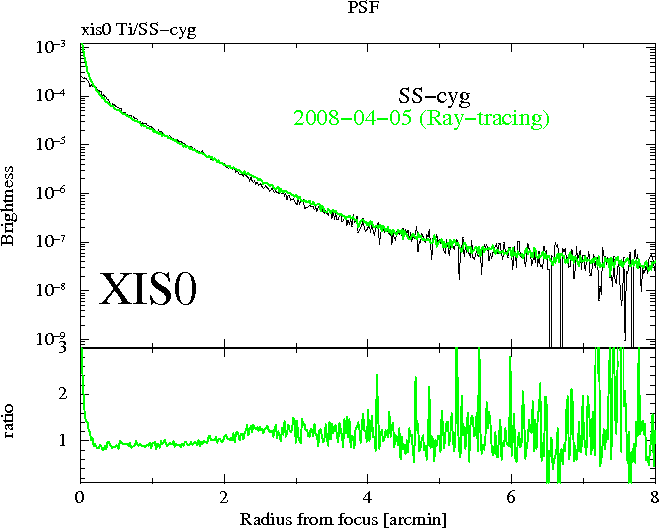
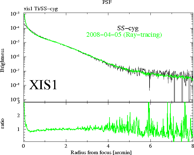
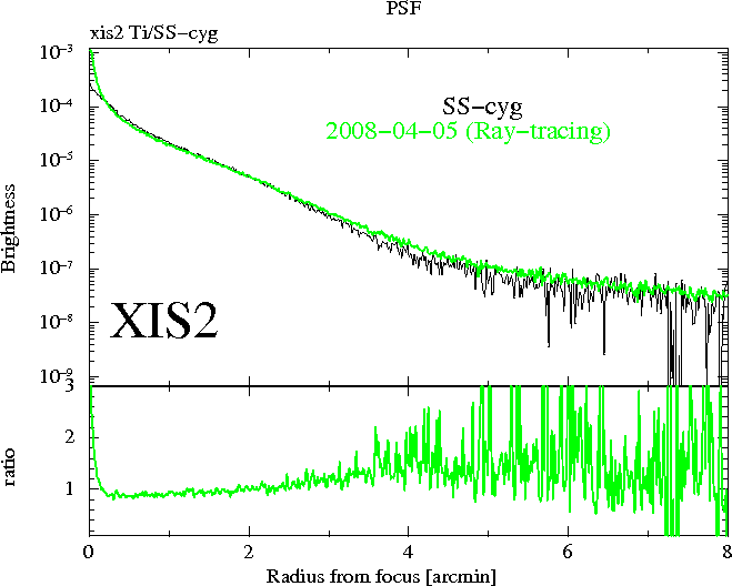
In Fig. 6.12, we show Point Spread Functions (PSFs) using the
data shown in Fig. 6.11 before smoothing. Note that the
core shape within ![]() is not tuned at all. The core broadening is
mainly due to the attitude error of the satellite control (Uchiyama et
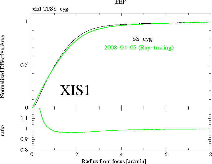
al. 2007). In Fig. 6.13, we show encircled energy functions
(EEFs). The reproducibility of the EEF is important when extracting
spectra from a circular region with a given radius. In the new
simulator, the EEF of the simulations coincides with that of the
observed data to within 4% for radii from 1
is not tuned at all. The core broadening is
mainly due to the attitude error of the satellite control (Uchiyama et
al. 2007). In Fig. 6.13, we show encircled energy functions
(EEFs). The reproducibility of the EEF is important when extracting
spectra from a circular region with a given radius. In the new
simulator, the EEF of the simulations coincides with that of the
observed data to within 4% for radii from 1![]() to 6
to 6![]() .
.
XIS0
|
|
|
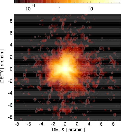
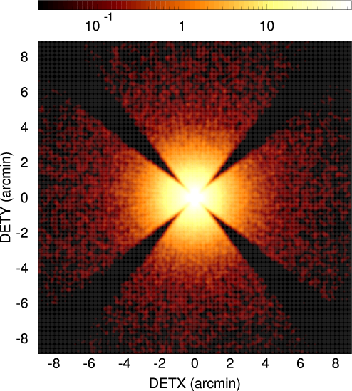
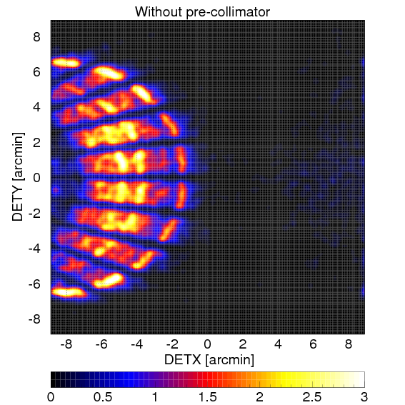
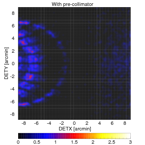
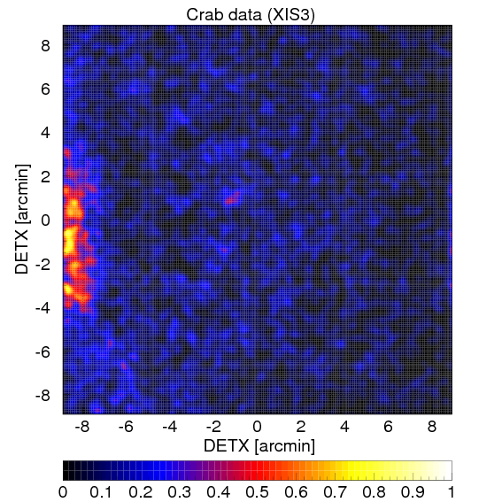
Studies of the stray light were carried out with Crab nebula off-axis pointings during 2005 August 22 - September 16 for a range of off-axis angles. An example of a stray light image is shown in the right panel of Fig. 6.14.
|
This image is taken with the XIS3 in the 2.5-5.5keV band with the
Crab nebula offset at ![]() in (DETX, DETY). The left and
central panels show simulated stray light images without and with the
pre-collimator, respectively, of a monochromatic point source of
4.5keV being located at the same off-axis angle. The ghost image
seen in the left half of the field of view is due to ``secondary
reflection''. Although ``secondary reflection'' cannot completely be
diminished at the off-axis angle of
in (DETX, DETY). The left and
central panels show simulated stray light images without and with the
pre-collimator, respectively, of a monochromatic point source of
4.5keV being located at the same off-axis angle. The ghost image
seen in the left half of the field of view is due to ``secondary
reflection''. Although ``secondary reflection'' cannot completely be
diminished at the off-axis angle of ![]() , the center of the field of
view is nearly free of stray light. The semi-circular bright region in
the middle panel, starting at (DETX, DETY)
, the center of the field of
view is nearly free of stray light. The semi-circular bright region in
the middle panel, starting at (DETX, DETY)![]()
![]() ,
running through
,
running through ![]() (
(![]() ), where the image becomes fainter, and
ending up at
), where the image becomes fainter, and
ending up at
![]() , originates from the innermost secondary
reflector, because the space between the innermost reflector and the
inner wall of the telescope housing is much larger than the
reflector-reflector separation. This semi-circular bright region is
only marginally visible in the real Crab nebula image in the right
panel. Another remarkable difference between the simulation and the
real observation is the location of the brightest area; in the
simulation, the left end of the image (DETX
, originates from the innermost secondary
reflector, because the space between the innermost reflector and the
inner wall of the telescope housing is much larger than the
reflector-reflector separation. This semi-circular bright region is
only marginally visible in the real Crab nebula image in the right
panel. Another remarkable difference between the simulation and the
real observation is the location of the brightest area; in the
simulation, the left end of the image (DETX
![]() ,
,
![]() ) is relatively dark whereas the
corresponding part is brightest in the Crab nebula image. These
differences originate from relative alignments among the primary and
secondary reflectors, and the blades of the pre-collimator, which are
to be calibrated by referring to the data of the stray light
observations in the near future.
) is relatively dark whereas the
corresponding part is brightest in the Crab nebula image. These
differences originate from relative alignments among the primary and
secondary reflectors, and the blades of the pre-collimator, which are
to be calibrated by referring to the data of the stray light
observations in the near future.
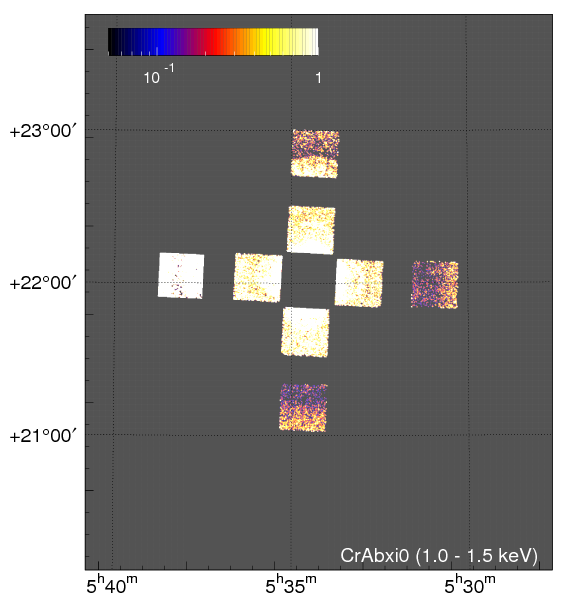
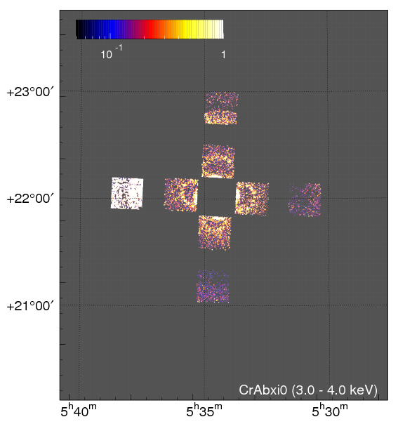
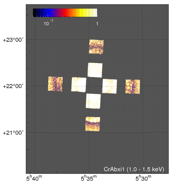
Overall, in-flight stray light observations of the Crab were carried
out with off-axis angles of ![]() (4 pointings),
(4 pointings), ![]() (4 pointing)
and
(4 pointing)
and ![]() (4 pointing) in 2005 autumn. Follow-up observations
covering more offset angles of
(4 pointing) in 2005 autumn. Follow-up observations
covering more offset angles of ![]() (4 pointing) ,
(4 pointing) , ![]() (8 pointing)
were made in 2010 autumn. Examples of mozaic images made with the
offset observations in SKY coordinate are shown in
Figures 6.15 and 6.16.
The stray images differ from offset to offset and from azimuth to
azimuth in the XRT coordinate. It also strongly depends on energy.
(8 pointing)
were made in 2010 autumn. Examples of mozaic images made with the
offset observations in SKY coordinate are shown in
Figures 6.15 and 6.16.
The stray images differ from offset to offset and from azimuth to
azimuth in the XRT coordinate. It also strongly depends on energy.
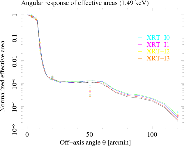
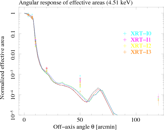
Figure 6.17 shows the measured and simulated angular
responses of the XRT-I at 1.5 and 4.5keV up to 2![]() . The
effective area is normalized to 1 at the on-axis position. The
integration area corresponds to the detector size of the XIS
(
. The
effective area is normalized to 1 at the on-axis position. The
integration area corresponds to the detector size of the XIS
(
![]() ). The plots are necessary to plan observations
of diffuse sources or faint emissions near bright sources, such as
outskirts of cluster of galaxies, diffuse objects in the Galactic
plane, SN 1987A, etc.. The four solid lines in the plots correspond to
raytracing simulations for the different detectors, while the crosses
are the normalized effective area using the Crab pointings. For
example, the effective area of the stray light at 1.5keV is
). The plots are necessary to plan observations
of diffuse sources or faint emissions near bright sources, such as
outskirts of cluster of galaxies, diffuse objects in the Galactic
plane, SN 1987A, etc.. The four solid lines in the plots correspond to
raytracing simulations for the different detectors, while the crosses
are the normalized effective area using the Crab pointings. For
example, the effective area of the stray light at 1.5keV is
![]() 10
10![]() at off-axis angles smaller than 70
at off-axis angles smaller than 70![]() and
and ![]() at off-axis angles larger than 70
at off-axis angles larger than 70![]() . The measured stray light flux is
in agreement with that of the simulations to within an order of
magnitude. The solution of the solid lines is incorporated into the
xissim and the xissimarfgen tools using CALDB 2008-06-02.
. The measured stray light flux is
in agreement with that of the simulations to within an order of
magnitude. The solution of the solid lines is incorporated into the
xissim and the xissimarfgen tools using CALDB 2008-06-02.
 |
For feasibility studies of XIS data analyses of faint objects near bright sources, proposers are encouraged to simulate observations using xissim in order to determine whether the stray light flux might dominate that of the faint object or not. Proposers who do observe a target heavily suffering from stray light contamination need to handle the data with special care regarding calibration errors. Faint objects in the Galactic center and plane often suffer from stray light contamination from bright X-ray stars, and the flux of the outskirts of galaxy clusters, widely extended over the detector field of view, is sometimes dominated by stray light from the bright core.
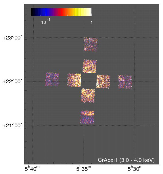
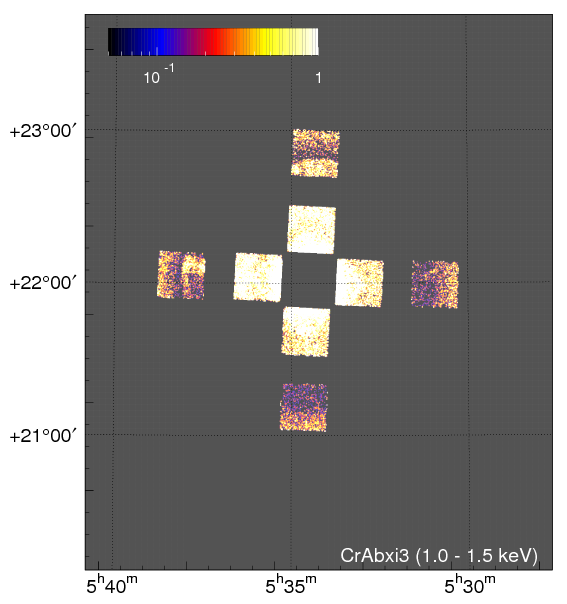
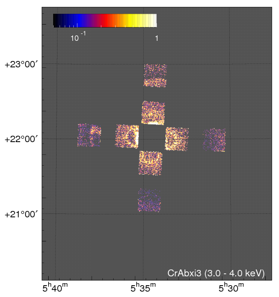
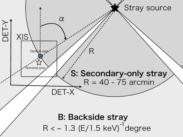
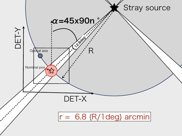
Observers can avoid contamination from stray light if they choose the
roll and offset angles properly. Fig. 6.18 shows a
schematic diagram of the stray light patterns for a stray light source
at an azimuth angle of ![]() and an offset angle of
and an offset angle of ![]() . The square
in Fig. 6.18 corresponds to the XIS field of view. The
nominal position is located within 1 arcmin from the optical axis of
the XIS system within a couple of arcmins. The XIS field of view near
to and far from a stray light source is contaminated by stray light of
the ``Secondary-reflection component'' and the ``Backside component'',
respectively (Mori et al. 2005, PASJ 57, 245). On the other hand the
near and far sides are free from the ``Backside component'' and the
``Secondary-reflection component'', respectively. There is another
stray light free region corresponding to the ``Quadrant Boundary''
with a cone angle of 12.8 deg at an azimuth angle of 45 deg with 90
deg pitch. Observers can thus choose between three kinds of the
``stray light free'' regions. Fig. 6.19 shows pointing
positions targeting these three kinds of stray light free regions,
marked in white: the ``Quadrant Boundary'' region (top), the ``
Secondary-reflection component free'' region (middle) and the
``Backside component free'' region (bottom).
. The square
in Fig. 6.18 corresponds to the XIS field of view. The
nominal position is located within 1 arcmin from the optical axis of
the XIS system within a couple of arcmins. The XIS field of view near
to and far from a stray light source is contaminated by stray light of
the ``Secondary-reflection component'' and the ``Backside component'',
respectively (Mori et al. 2005, PASJ 57, 245). On the other hand the
near and far sides are free from the ``Backside component'' and the
``Secondary-reflection component'', respectively. There is another
stray light free region corresponding to the ``Quadrant Boundary''
with a cone angle of 12.8 deg at an azimuth angle of 45 deg with 90
deg pitch. Observers can thus choose between three kinds of the
``stray light free'' regions. Fig. 6.19 shows pointing
positions targeting these three kinds of stray light free regions,
marked in white: the ``Quadrant Boundary'' region (top), the ``
Secondary-reflection component free'' region (middle) and the
``Backside component free'' region (bottom).
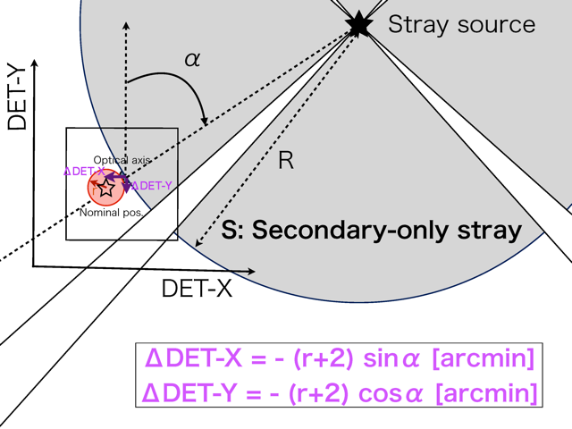
![]() DET-X
DET-X ![]()
![]() [arcmin]
[arcmin]
![]() DET-Y
DET-Y ![]()
![]() [arcmin].
[arcmin].
Note that the offset direction is towards the near side of the stray
light source. The margin of 2 arcmin corresponds to the misalignment
between the optical axis and the nominal position. The Backside
component appears within an offset angle ![]() of up to
of up to
![]() (
(![]() 1.5keV). If the stray
light source is located further away than the critical offset angle,
observers can choose the Secondary-reflection component free region,
as well.
1.5keV). If the stray
light source is located further away than the critical offset angle,
observers can choose the Secondary-reflection component free region,
as well.
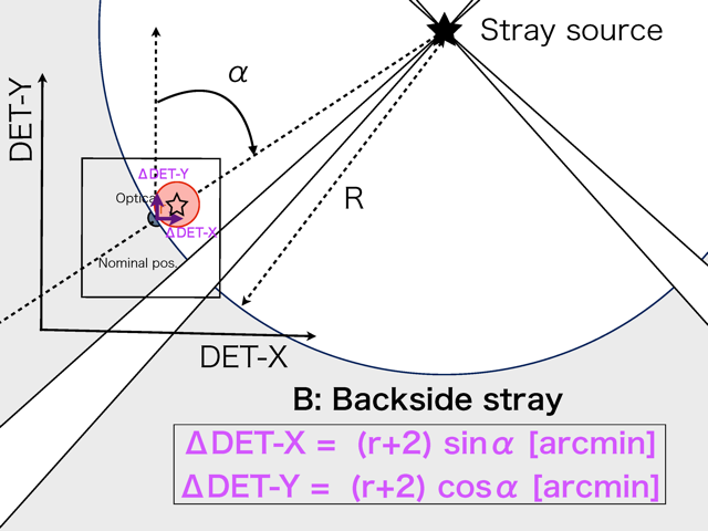
![]() DET-X
DET-X ![]()
![]() [arcmin]
[arcmin]
![]() DET-Y
DET-Y ![]()
![]() [arcmin].
[arcmin].
The offset direction is towards the far side of the stray light source.
If observers cannot choose any of the three stray light free regions, the possibility of contamination through stray light exists.
|