XMM-Newton Science Analysis System: User Guide

Next: 4.12.2.2 Inspection of spectra or timeseries using the command line Up: 4.12.2 Example of EPIC product generation: images, spectra & light curves Previous: 4.12.2 Example of EPIC product generation: images, spectra & light curves

4.12.2.1 Working from the command line

The user can perform the described analysis with command lines by executing the following steps:

In order to avoid long names and path, it might be convenient to first define the name of the input calibrated event list as a variable:

set evfile=/path to PPS directory/P0123700401PNS003PIEVLI0000.FIT

where as an example the pn event list from the pipeline processing of the public Lockman Hole data set is shown.

Create a light-curve for the observation to check for flaring high background periods (which are best visible above 10 keV):
```
evselect table=$evfile withrateset=yes rateset=rates.fits \
         timecolumn=TIME timebinsize=100 \
         makeratecolumn=yes maketimecolumn=yes \
         expression='#XMMEA_EP && PI in [10000:12000] && (PATTERN==0)'
```
Note, in case of MOS #XMMEA_EM && PI > 10000 && (PATTERN==0) shall be used.
Plot the light-curve (see figure 26):
```
dsplot table=rates.fits x=TIME y=RATE &
```
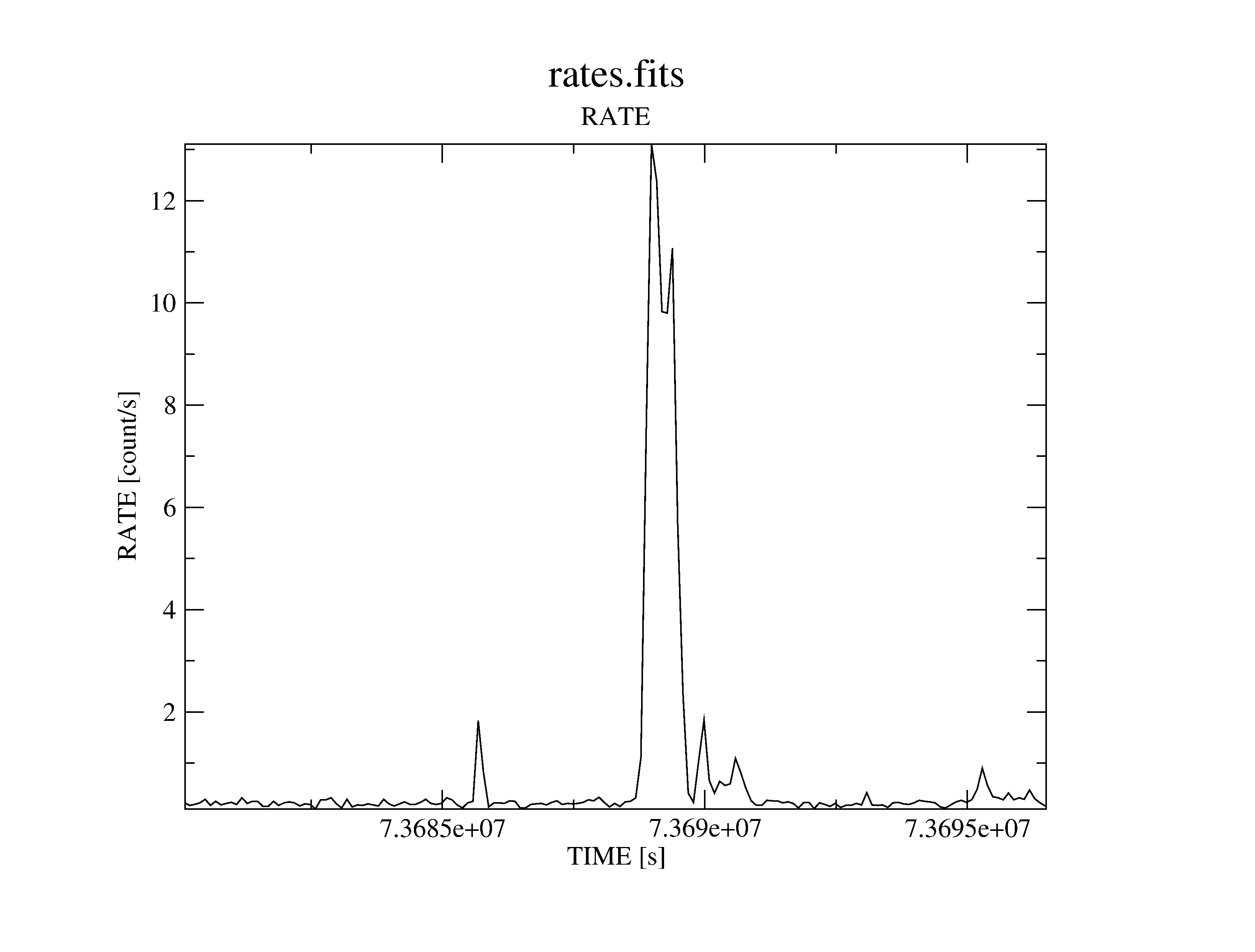Figure 26: Light-curve of the example data set. Flaring high background periods are clearly visible.
$\begin{figure}\centerline{\psfig{figure=EPIC/lightcurve_total_rate.ps,width=18cm,clip}}\end{figure}$

Determine a threshold on the light-curve, defining low background intervals (in our example: 0.4 counts/s) and create a corresponding good time interval (GTI) file:
```
tabgtigen table=rates.fits expression='RATE<=0.4' gtiset=gti.fits
```
Note: the recommended cut value for MOS observations is 0.35 counts/s but the choice of the thresholds strongly depends on the science the user is interested in.
Create an event list which is free of high background periods. Also this might be the place to restrict the further analysis to the well calibrated patterns and energy band:
```
evselect table=$evfile withfilteredset=true filteredset=filtered.fits \
         keepfilteroutput=true destruct=true \
         expression='(gti(gti.fits,TIME) && (PI in [100:15000]) && (PATTERN<=4))'
```
Note, in case of MOS (PATTERN<=12) shall be used. Create a new light curve to make sure that the flaring background time intervals were removed:
```
evselect table=filtered.fits withrateset=yes rateset=rates_new.fits \
         timecolumn=TIME timebinsize=100 maketimecolumn=yes \
         makeratecolumn=yes expression='#XMMEA_EP \
         && PI in [10000:12000] && (PATTERN==0)'
```
Note, in case of MOS #XMMEA_EM && PI > 10000 && (PATTERN==0) shall be used.
Plot the new light-curve (see figure 27):
```
dsplot table=rates_new.fits x=TIME y=RATE &
```
Figure 27: Light-curve of the example data set after removal of flaring high background periods.
$\begin{figure}\centerline{\psfig{figure=EPIC/lightcurve_clean_rate.ps,width=18cm,clip}}\end{figure}$

From now on, the filtered events file (filtered.fits) will be used for further analysis. In the case of the example data set, the number of events in the filtered event list is less the half of what the original event list had, a fact which will speed up further processing significantly. The size of the event list (especially in case of bright sources) can be further reduced a lot by also excluding the following columns: RAWX/Y, DETX/Y, PHA.
Create a sky image of the filtered data set:
```
evselect table=filtered.fits withimageset=true imageset=image.fits \
         xcolumn=X ycolumn=Y \
         imagebinning=binSize ximagebinsize=80 yimagebinsize=80
```
and display the image with ds9:
```
ds9 image.fits &
```
The parameter settings imagebinning=binSize and x/yimagebinsize=80 bin the image into squared pixels of $80\times0.05=4$ arcsec (0.05 arcsec being the unit of the X, Y sky coordinate system).
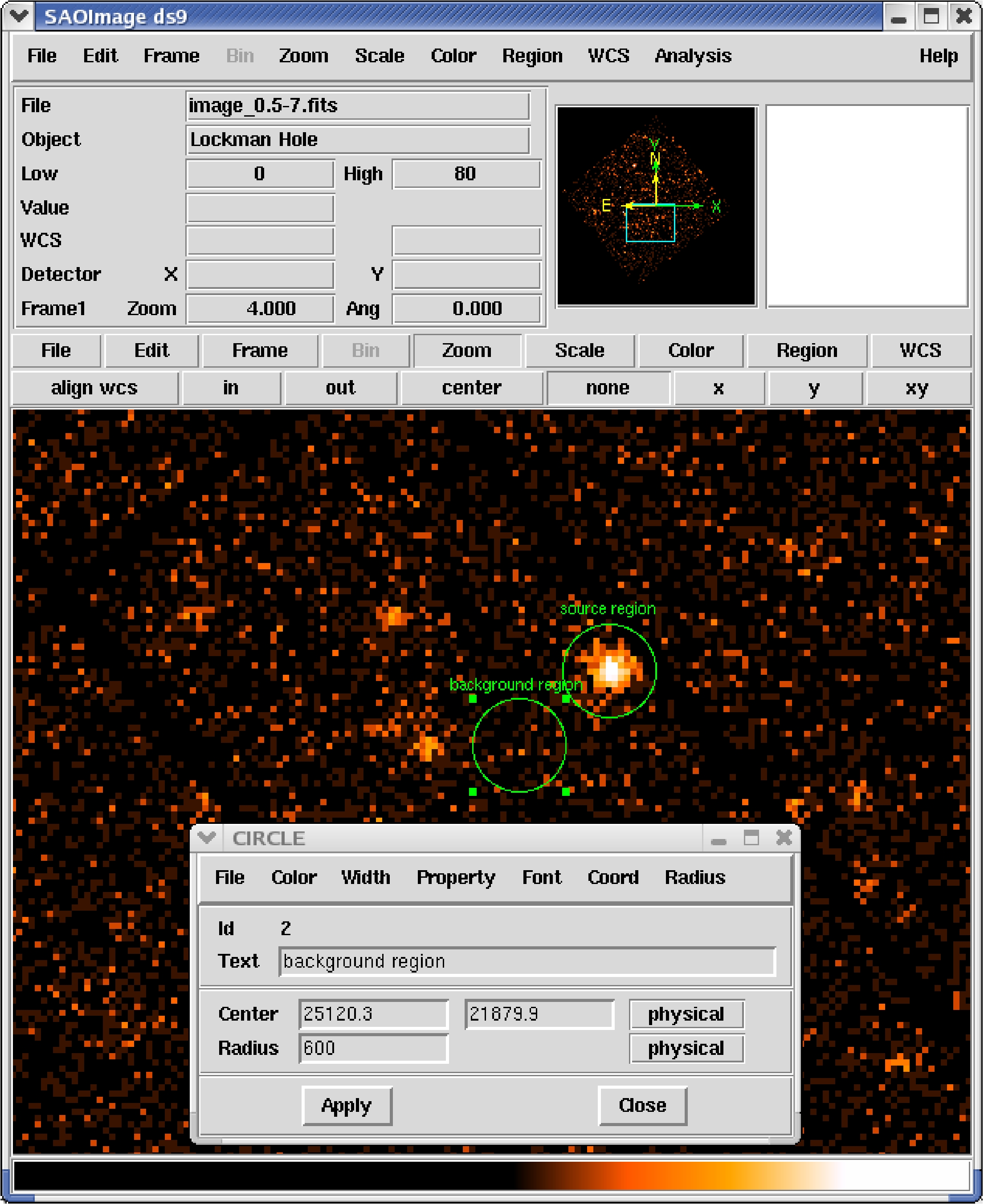
Specifying an additional selection expression of the form expression='PI in [..:..]' allows creation of images in different energy bands, e.g., figure 28 shows the image in the energy range 0.5-7 keV.

Figure 28: Sky image of the example data set in the energy range 0.5-7 keV displayed with ds9.
$\begin{figure}\centerline{\psfig{figure=EPIC/image_0.5-7.ps,width=12cm}}\end{figure}$
Extract source and background spectra for a bright point-like field source: in the displayed image a region around the source can be selected by positioning the cursor on the source center. Keeping the left mouse button pressed, the size of the circular extraction region can be changed. Clicking after-wards again on the region selects it. With the left mouse button the position and size of the region can interactively be changed. It is also possible to change characteristic region parameters via double clicking on the region as well as to save a region via the "Region/Save Regions..." menu in ds9.
To apply the specified region as a spatial filter expression in evselect, the properties of the region need to be given in physical sky coordinates. To do this, make sure that the coordinates and radius are displayed in physical units in the selection region properties window.
In our example, the spatial selection expression for the source spectrum is (X,Y) IN circle(26285.6,22842.1,600). The extraction radius is 30 arcsec. The same values would also be propagated into the selection expression by pressing the "2D Region" button in xmmselect.
The source spectrum is extracted with the following command line:
```
evselect table=filtered.fits withspectrumset=yes \
         spectrumset=spectrum.fits energycolumn=PI \
         withspecranges=yes specchannelmin=0 specchannelmax=20479 \
         spectralbinsize=5 \
         expression='((X,Y) IN circle(26285.6,22842.1,600)) && \
                     (FLAG==0) && (PATTERN<=4)'
```
Parameters specchannelmax=20479 and spectralbinsize=5 are the recommended settings for a pn data set. In the case of MOS data, they should be set to
specchannelmax=11999 and spectralbinsize=5. This setup allows the optional usage of the "canned" response matrices.
Including (FLAG==0) in the selection expression is recommended for pn. This selection is even more restrictive than the #XMMEA_EP event attribute flag as it rejects, in addition, events which are close to CCD gaps or bad pixels. In the case of MOS, the filter expression #XMMEA_EM might be sufficient.
For pn the spectral analysis is restricted to the better calibrated single and double events ((PATTERN<=4)). In the case of MOS, all valid patterns ((PATTERN<=12)) might be included.
The source spectrum can be displayed with the following command:
```
dsplot table=spectrum.fits &
```
In a next step, one needs to extract a background spectrum:
In our pn example the source is located close to the edge of a CCD at a RAWY position of about 138. A surrounding annulus for the background extraction would include the CCD gap and eventually also part of a neighboring CCD. Hence in this case it might be better to define the background via a circle on the same CCD where the source is located at roughly the same distance from the readout node (same RAWY as the source) placed in a source free region (see figure 29 for the selected source and background regions parameters):
```
evselect table=filtered.fits withspectrumset=yes \
         spectrumset=background.fits energycolumn=PI \
         withspecranges=yes specchannelmin=0 specchannelmax=20479 \
         spectralbinsize=5 \
         expression='((X,Y) IN circle(25120.3,21879.9,600)) && \
                     (FLAG==0) && (PATTERN<=4)'
```
Figure 29: Selection regions for the extraction of source and background spectra.
$\begin{figure}\centerline{\psfig{figure=EPIC/extraction_regions.ps,width=12cm}}\end{figure}$

The background spectrum can be displayed again with the following command:
```
dsplot table=background.fits &
```
In the next step, the area of the extraction regions used to make the source and background spectral files must be calculated taking into account CCD boundaries and bad pixels. The area is written into the header of the SPECTRUM table of the input file as the keyword BACKSCAL:
```
backscale spectrumset=spectrum.fits badpixlocation=filtered.fits

backscale spectrumset=background.fits badpixlocation=filtered.fits
```
Note, if spectra are created via the xmmselect task, backscale will have automatically been applied "on the fly" during the product generation process.
Create response matrix files (Redistribution Matrix File (RMF) and Ancillary Response File (ARF)) using the rmfgen and arfgen tasks:
```
rmfgen spectrumset=spectrum.fits rmfset=spectrum.rmf
```
An alternative approach to obtain a RMF file is to use the ready-made "canned" response matrices available from the rmf files at the EPIC Response Files page ( http://www.cosmos.esa.int/web/xmm-newton/epic-response-files)
```
arfgen spectrumset=spectrum.fits arfset=spectrum.arf \
       withrmfset=yes rmfset=spectrum.rmf \
       badpixlocation=filtered.fits
```
Note, arfgen reads the pattern range from the data subspace (DSS) information in the spectrum dataset, and accumulates the quantum efficiency curves over those patterns, which are then combined to the other constituents of the ARF. Be aware that the entire range of allowed patterns (0-12 for the pn and 0-31 for the MOS, respectively) are assumed if no pattern range was found in the DSS.
Alternatively, make use of the especget meta-task to perform spectral analysis steps 4 and 5 in one go
Assuming that the user wants to use the same extraction regions for the source and background spectra as given above, the generation of spectra and related response files can be performed in one go with the following command:
```
especget table=filtered.fits filestem=mysource \
         srcexp='(X,Y) IN circle(26285.6,22842.1,600)' \
         backexp='(X,Y) IN circle(25120.3,21879.9,600)'
```
By default the following event selection is added to the spatial selection expressions: for pn (FLAG==0)&&(PATTERN<=4) and for MOS #XMMEA_EM&&(PATTERN<=12). The spectra are generated with spectral ranges and binnings automatically set in a way that canned response matrices (§ 4.8.2) could be used. The computation of the area of the extraction regions is performed "on the fly". In addition, especget writes the names of the created files into the source spectrum header keywords BACKFILE, RESPFILE, ANCRFILE. These may be automatically read by spectral fitting programmes to link the files and perform area weighted background subtraction.
The parameter filestem defines the names of the produced output files. In the example given above, especget generates the following output files:
- mysource_src.ds: the source spectrum
- mysource_bgd.ds: the background spectrum
- mysource_src.arf: the source related Ancillary Response File (ARF)
- mysource_src.rmf: the source related Redistribution Matrix File (RMF)
Note, if xmmselect is used to generate "OGIP Spectral Products" (see § 4.8.1), the user can interactively define source and background regions and (before especget is started) a source region optimization is performed via the task eregionanalyse (see 4.7.6).
Prepare the spectra for further analysis with Xspec
The task specgroup can be used to rebin the the spectrum. In the following example the spectrum is rebinned in order to have at least 25 counts for each background-subtracted spectral channel and not to oversample the intrinsic energy resolution by a factor larger then 3:
```
specgroup spectrumset=spectrum.fits mincounts=25 oversample=3 \
    rmfset=spectrum.rmf arfset=spectrum.arf \
    backgndset=background.fits
```
If the source spectrum was not generated with especget, the specgroup also offers the possibility to fill the keywords RESPFILE, ANCRFILE, and BACKFILE in the header of the spectral file. This is mandatory if users want to load the spectral file into XSPEC versions later then 12 for further analysis (as in the example given above).

**Figure 26:** Light-curve of the example data set. Flaring high background periods are clearly visible.
$\begin{figure}\centerline{\psfig{figure=EPIC/lightcurve_total_rate.ps,width=18cm,clip}}\end{figure}$

**Figure 27:** Light-curve of the example data set after removal of flaring high background periods.
$\begin{figure}\centerline{\psfig{figure=EPIC/lightcurve_clean_rate.ps,width=18cm,clip}}\end{figure}$

**Figure 28:** Sky image of the example data set in the energy range 0.5-7 keV displayed with `ds9`.
$\begin{figure}\centerline{\psfig{figure=EPIC/image_0.5-7.ps,width=12cm}}\end{figure}$

**Figure 29:** Selection regions for the extraction of source and background spectra.
$\begin{figure}\centerline{\psfig{figure=EPIC/extraction_regions.ps,width=12cm}}\end{figure}$

Create a light-curve for the source:

evselect table=filtered.fits withrateset=yes \
         rateset=lightcurve.fits timecolumn=TIME timebinsize=1 \
         expression='((X,Y) IN circle(26285.6,22842.1,600))'

The Xronos programme package can now be used to produce a binned light-curve, to calculate a power spectrum, search for periodicities etc.

The data analysis based on command lines was described here, as well as combining command lines into a script which might offer a good method for further re-performing of (part of) a data analysis session (see § 3.1 for a discussion of possible advantages of a GUI based analysis).

European Space Agency - XMM-Newton Science Operations Centre