---

THE XMM-NEWTON ABC GUIDE, STREAMLINED
RGS, SAS GUI

---

Contents

Prepare the Data
Reprocess the Data
Introduction to xmmselect
Make Images
Make a Light Curve
Generate and Apply a New GTI File
Check for Pile Up
Create the Photon Redistribution Matrix (RMF)
Combining Spectra

---

Prepare the Data

Please note that the two tasks in this section (cifbuild and odfingest) must be run in the ODF directory. These are the only tasks with that requirement, and after this section, we will work exclusively in our reprocessing directory.

Many SAS tasks require calibration information from the Calibration Access Layer (CAL). Relevant files are accessed from the set of Current Calibration File (CCF) data using a CCF Index File (CIF).

To make the ccf.cif file, first make sure the environment variables are set:

   cd ODF
   setenv SAS_ODF /full/path/to/ODF/directory/
   setenv SAS_ODFPATH /full/path/to/ODF/directory/

Next, call cifbuild from the SAS GUI. A window with the parameter options will appear; the defaults should be fine, so just click "Run".

To use the updated CIF file in further processing, you will need to reset the environment variable SAS_CCF:

   setenv SAS_CCF /full/path/to/ODF/ccf.cif

The task odfingest extends the Observation Data File (ODF) summary file with data extracted from the instrument housekeeping data files and the calibration database. It is only necessary to run it once on any dataset, and will cause problems if it is run a second time. If for some reason odfingest must be rerun, you must first delete the earlier file it produced. This file largely follows the standard XMM naming convention, but has SUM.SAS appended to it. After running odfingest, you will need to reset the environment variable SAS_ODF to its output file. To run odfingest and reset environment variable, call odfingest from the SAS GUI. As before, a pop-up window with the parameter options will appear; the defaults should be fine, so just click "Run". (It is safe to ignore the warnings.)

To change the environmental variable, type

   setenv SAS_ODF /full/path/to/ODF/full_name_of_*SUM.SAS

You will likely find it useful to alias these environment variable resets in your login shell (.cshrc, .bashrc, etc.).

Reprocess the Data

To reprocess the data, make a new working directory and call rgsproc from inside it.

   cd ..
   mkdir PROC
   cd PROC

Then, close and re-open the SAS GUI, so that it will place the output files in the new directory, and call rgsproc. The defaults are fine for most observations, so just click "Run". (It is safe to ignore the warnings.) This takes several minutes, and outputs 12 files per RGS, plus 3 general use FITS files. At this point, renaming files to something easy to type is a good idea.

    cp *R1*EVENLI*FIT r1_evt1.fits
    cp *R2*EVENLI*FIT r2_evt1.fits 

The pipeline task rgsproc is very flexible and can address potential pitfalls for RGS users. If the default parameters are sufficient for your data (and they should be for most), feel free to skip ahead. However, there are some cases where the standard processing may not be appropriate. These are discussed next.

My data has a bright optical source near the target!

First, if the data includes a nearby bright optical source, with certain pointing angles, zeroth-order optical light may be reflected off the telescope optics and onto the RGS CCD detectors. If this falls on an extraction region, the current energy calibration will require a wavelength-dependent zero-offset. Stray light can be detected on RGS DIAGNOSTIC images taken before, during and after the observation. This test, and the offset correction, are not performed on the data before delivery. Please note that this will not work in every case. If a source is very bright, the diagnostic data that this relies on may not have been downloaded from the telescope in order to save bandwidth. Also, the RGS target itself cannot be the source of optical photons, as the spectrum's zero-order falls far from the RGS chip array. To check for stray light and apply the appropriate offsets, invoke rgsproc in the GUI. Then,

1. In the "events" tab, under the "rgsoffsetcalc" sub-tab, set calcoffsets to yes.
2. Click "Run".

My data has a bright X-ray source near the target!

If the data includes a nearby bright X-ray background source that is well-separated from the target in the cross-dispersion direction, a mask can be created that excludes it from the background region. Here the source has been identified in the EPIC images and its coordinates have been taken from the EPIC source list which is generated by the task edetect_chain (see the EPIC walkthrough for more information). The bright neighboring object is found to be the third source listed in the sources file. The first source is the target. Invoke rgsproc in the GUI. Then,

1. In the "events" tab, under the "rgssources" sub-tab, set withepicset to yes and epicset to the name of the EPIC source list as generated by edetect_chain.
2. In the "spectra" tab, under the "rgsregions" sub-tab, set exclsrcsexpr to INDEX==1&&INDEX==3.
3. Click "Run".

I want to define my own target.

If the true coordinates of an object are not included in the EPIC source list or the science proposal, the user can define the coordinates of a new source. Call rgsproc in the GUI and then,

1. In the "events" tab, under the "rgssources" sub-tab, set withsrc to yes. Be sure that the box beneath withsrc is toggled to radec. Next to srcra, enter the RA in decimal degrees, 166.113808 and next to srcdec, enter the declination (again in decimal degrees), +38.208833. Next to srclabel, enter 'Mkn421'.
2. Click "Run".

Introduction to xmmselect

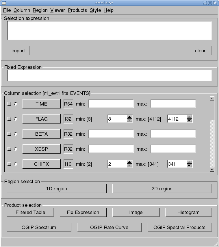
The task xmmselect is used for many procedures in the GUI. Like all tasks, it can easily be invoked by starting to type the name and pressing enter when it is highlighted.

When xmmselect is invoked a dialog box will first appear requesting a file name. You can either use the browser button or just type the file name in the entry area, "r1_evt1.fits:EVENTS" in this case. To use the browser, select the file folder icon; this will bring up a second window for the file selection. Choose the desired event file, then the "EVENTS" extension in the right-hand column, and click "OK". The directory window will then disappear and you can click "Run" on the selection window.

When the file name has been submitted the xmmselect GUI will appear, along with a dialog box offering to display the selection expression; this is shown in Figure 1. The selection expression will include the filtering done to this point on the event file, which for the pipeline processing includes for the most part CCD and GTI selections.

Different event files can be loaded into xmmselect by going to "File -> New Table".

Make Images

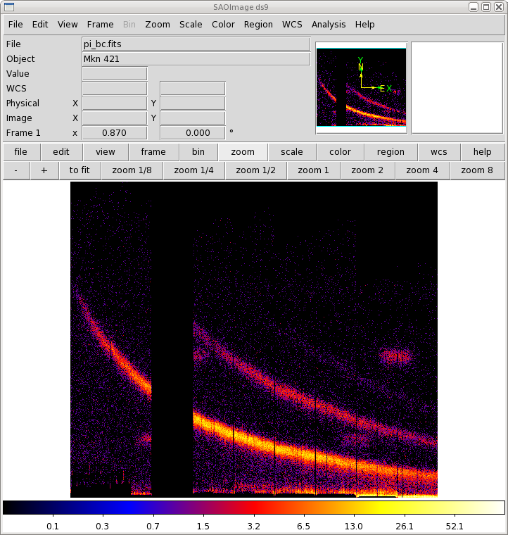
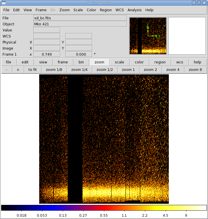
Two commonly-made plots are those showing PI vs. BETA_CORR (also known as "banana plots") and XDSP_CORR vs. BETA_CORR.

To make a banana plot, invoke xmmselect in the SAS GUI and load the event file r1_evt1.fits, as discussed above. Then,

1. Check the square boxes to the left of the BETA_CORR and PI entries to set the X and Y values in the image.
2. Click on the "Image" button near the bottom of the page. This brings up the evselect GUI.
3. Click on the "Image" tab in the evselect GUI. In the imageset box, enter the name of the output file. We will use pi_bc.fits.
4. Click "Run".

Different binnings and other selections can be found through options in the "Image" tab at the top of the GUI. The default settings are reasonable, however, for a basic image. The resultant image is automatically displayed using ds9. Plots comparing BETA_CORR to XDSP_CORR can be made in a similar way. These two example plots can be seen in Figure 2.

Make a Light Curve

The XMM-Newton Observatory is susceptible to soft particle flaring, so it is necessary to examine the light curve to determine how much of the data is useful. We will extract a region, CCD9, that is most susceptible to these events and generally records the least source events due to its location close to the optical axis. Also, to avoid confusing background for source variability, a region filter that removes the source from the final event list should be used. The region filters are kept in the source file product P*SRCLI_*.FIT.

More experienced users should be aware that with SAS 13, the *SRCLI* file's column information changed. rgsproc now outputs an M_LAMBDA column instead of BETA_CORR, and M_LAMBDA should be used to generate the light curve. (The *SRCLI* file that came with the PPS products still contains a BETA_CORR column if you prefer to use that instead.)

To make a light curve, call xmmselect from the GUI. Then,

1. Enter the filtering criteria in the "Selection expression" box: (CCDNR==9)&&(REGION(P0153950701R1S001SRCLI_0000.FIT:RGS1_BACKGROUND,M_LAMBDA,XDSP_CORR))
2. Check the round box to the left of the time entry.
3. Click on the "OGIP Rate Curve" button near the bottom of the page. This brings up the evselect GUI.
4. In the "Lightcurve" tab, change the timebinsize parameter to something reasonable, e.g. 10 or 100 s, and enter the output file name in the rateset box. We will use r1_ltcrv.fits.
5. Click "Run".

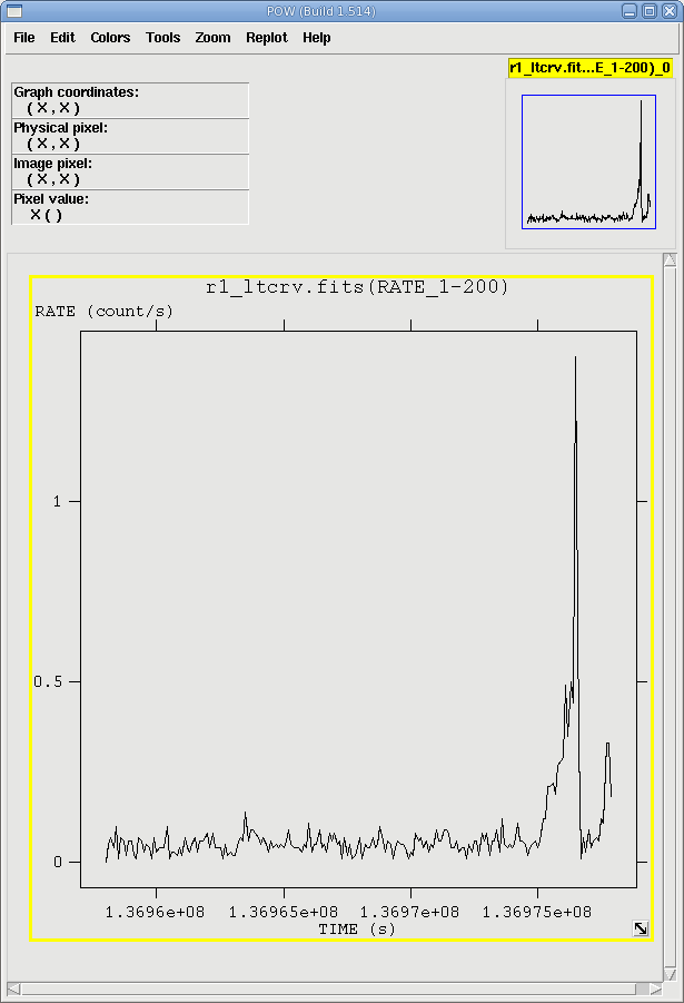
The resultant light curve is displayed automatically using Grace. It is shown in Figure 3.

Generate and Apply a New GTI File

Examination of the lightcurve shows that there is a loud section at the end of the observation, after 1.36975e8 seconds, where the count rate is well above the quiet count rate of about 0.05 count/second. To remove it, we need to make an additional Good Time Interval (GTI) file and apply it by rerunning rgsproc.

There are two tasks that make a GTI file: gtibuild and tabgtigen. Either will produce the needed file, so which one to use is a matter of the user's preference. Both are demonstrated below.

Filter on TIME With gtibuild

The first method, using gtibuild, requires a text file as input. In the first two columns, enter the start and end times (in seconds) that you are interested in, and in the third column, indicate with either a + or - sign whether that region should be kept or removed. Each good (or bad) time interval should get its own line. In the example case, we would write in our ASCII file (named gti.txt):

   1.36958e8 1.36975e8 +

and proceed to invoke gtibuild from the SAS GUI. Then,

1. For the file parameter, enter the name of the text file, gti.txt. For the table parameter, enter the output file name. We will use gti.fits.
2. Click "Run".

Filter on TIME With tabgtigen

Alternatively, we could filter on TIME with tabgtigen using the filtering expression from the good times noted previously. To do this, invoke tabgtigen from the SAS GUI, and then

1. In the table box, enter the name of the lightcurve file, r1_ltcrv.fits. In the gtiset box, enter the name of the output file; we will use gti.fits. In the expression box, enter the filtering expression: (TIME in [1.36958e8:1.36975e8])
2. Click "Run".

Filter on RATE With tabgtigen

Finally, we could filter on RATE using tabgtigen. The typical background count rate for this observation is about 0.05 ct/s, so we will use that in the filtering expression. Invoke tabgtigen from the SAS GUI, and then

1. In the table box, enter the name of the lightcurve file, r1_ltcrv.fits. In the gtiset box, enter the name of the output file; we will use gti.fits. In the expression box, enter the filtering expression. Since the nominal count rate is about 0.05 ct/s, we will set the upper limit to 0.05 ct/s: RATE < 0.05
2. Click "Run".

Apply the New GTI File

We can apply the GTI to the event file by running rgsproc again. rgsproc is a complex task, running several steps, with five different entry and exit points. It is not necessary to rerun all the steps in the procudure, only the ones involving filtering. Call rgsproc from the SAS GUI, then

1. In the "global" tab, set entrystage to 3:filter and finalstage to 5:fluxing.
2. In the "filter" tab, set auxgtitables to the new gti file, gti.fits.
3. Click "Run".

Remember to change the name to something easy to type.

   cp *R1*EVENLI*FIT r1_evt2.fits
   cp *R2*EVENLI*FIT r2_evt2.fits

Check for Pile Up

Depending on how bright the source is event pile up may be a problem. Pile up occurs when a source is so bright that incoming X-rays strike two neighboring pixels or the same pixel in the CCD more than once in a read-out cycle. In the RGS, it will cause two coincident 1^st order photons to combine into a single 2^nd order event at the same spatial position on the detector but at half the wavelength; this results in photons moving from 1^st order to 2^nd order, and 2^nd order to 3^rd. Further, it can increase the number of complicated event patterns of the sort that the on-board processing removes; this results in differences in pile up between the two RGS detectors, and between CCD locations.

It is always a good idea to check if your observation is piled up, especially if the object is bright (total count rate in all orders > 12 cts/s in RGS1, and 6 cts/s in RGS2).

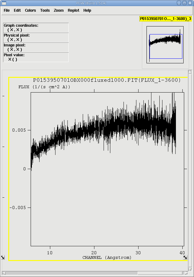
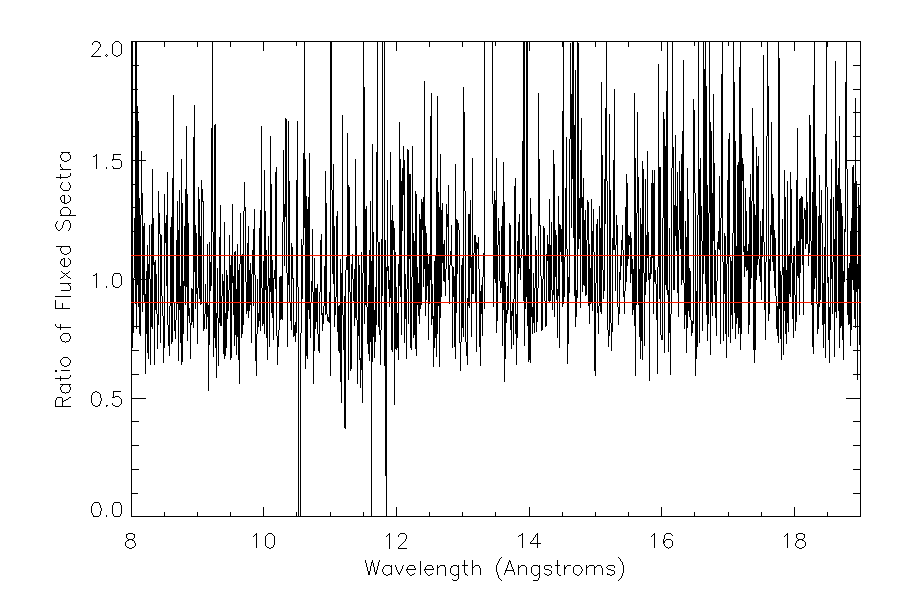
One way to determine if there is pile up is to examine the ratio of 1^st and 2^nd order fluxed spectra. Non-piled sources should have fluxed spectra that agree within a few percent, while piled sources will show discrepancies of about 10% or higher.

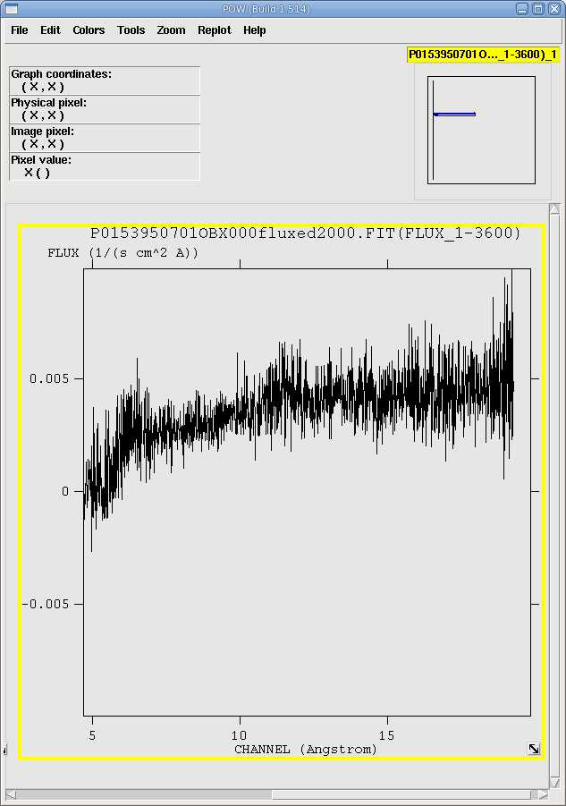
When rgsproc is run through the 5:fluxing stage, one of the outputs is fluxed spectra. They follow the naming convention *OBX*fluxed1000.FIT and *OBX*fluxed2000.FIT, for the 1^st and 2^nd orders, respectively. They can be viewed with fv, as in Figure 4.

If for some reason rgsproc wasn't run through that stage, fluxed spectra are easy enough to produce with rgsfluxer. Please note that rgsfluxer requires as input the response files (RMFs) for the spectra; these are produced by rgsproc (and have the nomenclature *RSPMAT*.FIT) or, alternatively, can be generated with the task rgsrmfgen as discussed below. Each RGS instrument and each order will have its own RMF.

To make a fluxed 1^st order spectrum, call rgsfluxer from the SAS GUI and then:

1. In the pha parameter, enter the names of the first order spectrum files, seperated by a space:
   P0153950701R1S001SRSPEC1001.FIT P0153950701R2S002SRSPEC1001.FIT
   In the rmf parameter, enter the names of the associated RMF files, again seperated by a space:
   P0153950701R1S001RSPMAT1001.FIT P0153950701R2S002RSPMAT1001.FIT
   In the file parameter, enter the output file name. We will use fluxed_o1.fits.
2. Click "Run".

Fluxed 2^nd order spectra are made in a similar way. The spectra are shown in Figure 4.

Unfortunately, if your spectrum is piled up, there is not a lot you can do to fix it; there is no tried-and-true method like with the EPIC and what there is applies only to certain cases, such as if you assume the 2^nd order spectrum is composed entirely of piled up 1^st order photons. For more information, see Ness et al. 2007, ApJ, 665, 1334.

Create the Photon Redistribution Matrix (RMF)

Response matrices (RMFs) are not provided as part of the pipeline product package (PPS); as noted above, rgsproc generates a response matrix automatically, with the nomenclature *RSPMAT*.FIT. But recall that the source coordinates are under the user's control. The source coordinates have a profound influence on the accuracy of the wavelength scale as recorded in the RMFs that are produced automatically by rgsproc.

Making the RMFs is easily done with rgsrmfgen. Please note that, unlike with EPIC data, it is not necessary to make ancillary response files (ARFs).

To make the RMFs, call rgsrmfgen from the GUI, then

1. In the spectrumset box, enter the name of the spectrum file; for RGS1, order 1, this would be P0153950701R1S001SRSPEC1001.FIT. In the evlist box, enter the name of the event list, r1_evt2.fits. Set emin to 0.4, emax to 2.5, and rows to 5000. Set rmfset to the output file name. We will use r1_o1_rmf.fits.
2. Click "Run".

RMFs for the RGS1 2^nd order, and for the RGS2 1^st and 2^nd orders, are made in a similar way.

At this point, the spectra can be either analyzed or combined with other spectra.

Combining Spectra

Spectra from the same order in RGS1 and RGS2 can be safely combined to create a spectrum with higher signal-to-noise if they were reprocessed using rgsproc with spectrumbinning=lambda. (This is the default setting.) The task we will use to merge source spectra, rgscombine, also merges response files and background spectra. When merging response files, be sure that they have the same number of bins. For this example, we will use the RMFs that were generated by rgsproc, which have a default bin number of 4000.

To merge the 1^st order RGS1 and RGS2 spectra, call rgscombine from the SAS GUI, and then

1. In the pha box, enter the spectrum files to combine, seperated by a space:
   P0153950701R1S001SRSPEC1001.FIT P0153950701R2S002SRSPEC1001.FIT
   In the bkg box, enter the corresponding background files:
   P0153950701R1S001BGSPEC1001.FIT P0153950701R2S002BGSPEC1001.FIT
   In the rmf box, enter the response files:
   P0153950701R1S001RSPMAT1001.FIT P0153950701R2S002RSPMAT1001.FIT
   
2. In the filepha box, enter the name of the output merged spectrum, r12_o1_srspec.fits. In the filermf box, enter the name of the output merged response files, r12_o1_rmf.fits. In the filebkg box, enter the name of the output merged background spectrum, r12_o1_bgspec.fits.
3. Confirm that the rmfgrid parameter to the same as that used to make the RMFs, 4000.
4. Click ``Run''.

The spectrum can be fit using HEASoft or CIAO packages, as SAS does not include fitting software.

---

If you have any questions concerning XMM-Newton send e-mail to xmmhelp@lists.nasa.gov

This file was last modified on Tuesday, 19-Nov-2013 17:08:40 EST
Curator:Michael Arida (ADNET); michael.arida@nasa.gov