---

The medium-energy concentrator spectrometer on board the BeppoSAX X-ray astronomy satellite

---

G. Boella^1,3, L. Chiappetti¹, G. Conti¹, G. Cusumano², S. Del Sordo², G. La Rosa², M.C. Maccarone², T. Mineo², S. Molendi¹, S. Re², B. Sacco², and M. Tripiciano²

• 1 CNR - Istituto di Fisica Cosmica e Tecnologie Relative, Via Bassini 15, 20133 Milano, Italy
• 2 CNR - Istituto di Fisica Cosmica ed Applicazioni dell'Informatica, Via Ugo La Malfa 153, 90146 Palermo, Italy
• 3 Dip. Fisica, Università di Milano, Via Celoria 16, 20133 Milano, Italy

Abstract

The scientific instrumentation on board the X-ray Astronomy Satellite BeppoSAX includes a Medium Energy Concentrator Spectrometer (MECS), operating in the energy range 1.3 - 10 keV, which consists of three units, each composed of a grazing incidence Mirror Unit and of a position sensitive Gas Scintillation Proportional Counter. The design and performance of the MECS instrument are here described, together with its on-ground calibration.

Key words: Instrumentation: detectors - X-rays: general

---

Introduction

The X-ray Astronomy Satellite BeppoSAX is a joint project of the Italian Space Agency (ASI) and the Netherlands Agency for Aerospace Programs (NIVR) devloped by a consortuim of institutes in Italy and The Netherlands, including the Space Science Department of ESA (SSD). BeppoSAX, with an expected lifetime of up 4 years, is devoted to systematic, integrated, and comprehensive studies of galactic and extra-galactic sources in the wide energy band 0.1 - 300 keV. The spacecraft, three axis stabilised and with a total mass of ~400 Kg, has bee launched by an Atlas G-Centaur on April 30, 1996, 04:31 GMT, into a circular equatorial orbit of ~3^oinclination and 600 Km altitude. The scientific payload comprises four Narrow Field Instruments NFI (Low Energy Concentrator Spectrometer LECS, Medium Energy Concentrator Spectrometer MECS, High Pressure Gas Scintillation Proportional Counter HPGSPC, Phoswich Detection System PDS) all pointing in the same direction, and two Wide Field Cameras WFC, pointing in diametrically opposed directions

---

Send offprint requests to: M.C. Maccarone: cettina@ifcai.pa.cnr.it

---

perpendicular to the NFI common axis. A detailed description of the entire BeppoSAX mission can be found in Butler & Scarsi (1990) and in Boella et al. (1996).

The MECS, operating in the medium X-ray energy band, is one of the NFI instruments onboard BeppoSAX. The main scientific objectives of the MECS are: spectroscopy from 1.3 to 10 keV (E / (D E_FWHM) in the range 6 - 16); imaging with angular resolution at the at the arcmin level; timing variabilty on time scales down to the millisecond. In this paper we give a description of the MECS instrument and its performance. Design, development, calibration and data analysis have been carried out by the MECS team at the IFCAI-Palermo and IFCTR-Milano Institutes in Italy, supported by the Italian Space Agency ASI in the framework of the BeppoSAX mission. The MECS on-ground calibration was performed at the X-ray PANTER facility of the Max Planck Institute, Germany; preliminary results of on-ground calibration analysis can be found in Boella et al. (1995) and in Molendi et al. (1995).

2. MECS description

The MECS consists of three units, each composed of a grazing incidence Mirror Unit (MU), and of a position sensitive Gas Scintillation Proportional Counter (GSPC) located at the focal plane. The MUs are connected to the GSPCs by a Carbon fiber envelop, about 2 m long. MECS overall performance is listed in Table 1. The quoted angular resolution values indicate the radii encircling 50% and 80% of the total signal, respectively (r₅₀, r₈₀).

2.1. Mirror unit

Each MU is composed of 30 nested coaxial and confocal mirrors. The mirrors have a double cone geometry to approximate the Wolter I configuration (Citterio et al., 1985), with diameters ranging from 68 to 162 mm, total

---

Table 1. MECS overall performance

Parameter	Value
Field of View	28' radius
Focal length	1.85 m
Angular resolution:
'' at 1.5 keV	r50=105" , r80=165"
'' at 6.4 keV	r50=75" , r80=150"
'' at 8.1 keV	r50=75" , r80=150"
Energy range	1.3 - 10 keV
Energy resolution	~8 (6/EkeV)½ % FWHM
Total on-axis effective area:
'' at 1.5 keV	31 cm2
'' at 6.4 keV	150 cm2
'' at 8.1 keV	101 cm2
Time resolution	15 micro sec
Image binning	256x256 pixels
Image pixel dimension	20" by 20" square
Energy binning	256 channels
Burst length binning	256 channels
Total maximum throughput	2000 cts/sec (4 Crab)

---

length of 300 mm, thickness from 0.2 to 0.4 mm and focal length of 1850 mm. The MU design was optimized to have the best response at 6 keV. A replica technique by nickel electroforming from super-polished mandrels was used to build up the mirrors (Citterio et al., 1988). A 1000 Å thick gold layer provides the X-ray reflecting surface. The 30 mirrors are nested using two front-end spiders with eight arms. The geometrical collecting area of each MU is 123.9 cm² ; the spiders and an active anti-ions grid reduce this geometrical area by about 18%. The measured radius for 50%, 80% and 90% encircled energy are of the order of 40, 110, and 210 arcsec at 8 keV, respectively. A more detailed description of the MU Point Spread Function can be found in Conti et al. (1993, 1994).

2.2. Detector unit

The focal plane detectors are Xenon filled GSPC, working in the range 1.3 -10 keV with an energy resolution of ~8% at 5.9 keV and a position resolution of ~0.5 mm (corresponding to 1 arcmin, aproximately) at the same energy. The gas cell is composed by a cylindrical ceramic body (96 mm internal diameter) closed, at the top, by a 50 ^-6m thick entrance Beryllium window with 30 mm diameter and, on the bottom, by an UV exit window made of Suprasil quartz with 80 mm diameter and 5 mm thickness, as schematically shown in Fig. 1. In flight, the getter can be activated to purify the gas, if necessary.

The entrance window is externally supported by a Beryllium strongback structure, 0.55 mm thick, consisting of a ring (10 mm inner diameter, 1 mm width) connected to the window border by four ribs, as shown in Fig. 2.

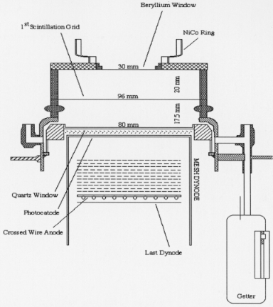Fig. 1. Schematic view of the MECS instrument: gas cell and position sensitive GSPC

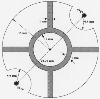Fig. 2. Geometry of the strongback

An X-ray photon absorbed in the gas cell liberates a cloud of electrons. A uniform electrical field across the cell drifts the cloud up to the scintillation region, with an higher electric field, where UV light is produced through the interaction of the accelerated electrons with the Xe ions. The amplitude of the UV signal, detected by a PMT, is proportional to the energy of the incident X-ray. The duration of the signal, the so-called Burst Length (BL), depends on the interaction point and it is used to discriminate genuine X-rays against induced background events. BL rejection may be carried out on board and/or onground. The BL rejection mechanism on board is based on a programmable BL acceptance window (not energy dependent). Two grids inside the cell separate the absorption/drift region (20 mm depth) from the scintillation region (17.5 mm depth). The UV readout system consists of a crossed-wire anode position sensitive Hamamatsu photomultiplier (PMT) with quantum efficiency of ~20%. The high voltage nominal values are -8 kV for the Be window, -7 kV for the scintillation grid, 1000, 992, and 943 V for the PMT of ME1, ME2, and ME3 units, respectively.

Two ⁵⁵Fe collimated calibration sources (nuclear line at 5.95 keV), with an emission rate of ~1 count per second, are located, diametrically opposed, near the edge of the Be window. These inner calibration sources, continuosly visible at the edge of the Field of View (FOV), allow the monitoring of the detector gain. Furthermore a passive ion shield is placed in front of the detector. The focal plane detector characteristics are shown in Table 2.

---

Table 2. Focal plane detector

Parameter	Value
Position resolution	0.7 (6/E)½ arcmin
Gas Type	Xenon
Gas filling pressure	1.0 atm at 25oC
X-ray window:
'' material	Beryllium
'' diameter	30.0 mm
'' thickness	50-6m
'' central region diameter	10 mm
'' support frame:
'' '' material	Beryllium
'' '' thickness	0.55 mm

---

2.3. Electronic unit

The MECS electronic processing takes place, almost entirely, in the Electronic Unit; only signal buffering is performed near the PMTs (one for each detector).

From each PMT, six signals are transferred to the Electronic Unit: Trigger, Energy, X ₁, X ₂, Y ₁1, and Y ₂2. All the signals are converted from current to voltage before to be passed to the Electronic Unit; in particular, the Energy and the position signals are integrated with a little time constant (few hundred of nanoseconds). The Trigger signal is taken from the 14^thdynode whereas the Energy is taken from the 15^thdynode (the last one). The X₁ and X₂ signals come out from the 16 anode wires (connected through a resistor divider) that give information about the X position. The same is valid for Y₁ and Y₂.

In the Electronic Unit there are three analog processing modules (one for each detector) followed by one Event Processor that arranges the data in packets sending them to the Communication Processor.

All the signals incoming from a single PMT (Trigger excepted) undergo to a baseline restoring and then they are integrated by Gated Integrators with fixed 25^-6s integration time. The X and Y positions are calculated (via hardware) from the original X₁, X₂, Y₁ and Y₂ in accordance to the formulas:

X = [X₁ - X₂] / [X₁ + X₂]

Y = [Y₁ - Y₂] / [Y₁ + Y₂]

The Burst length BL signal is obtained from the Energy through a constant fraction, zero crossing and Time-to-amplitude Converter chain.

There is a programmable selection logic, working on Energy and BL signals, to reject events before the A/D conversion. If during the integration time two trigger pulses are recognised, then the Pile-up Logic will reset the electronics in order to be ready for the next event. An Event Qualification Logic increments the Ratemeter registers, that are read at 1 s rate.

After the A/D conversion the data are saved into a FIFO register together with the event time. Data from the FIFO are read by the Event Processor and submitted to a rejection rule with programmable windows for Energy, BL, X and Y. Finally data are packed and written in a Dual Port RAM from where they will be read by the Communication Processor.

3. On-ground calibration set-up

The three flight MECS units have been extensively calibrated (~170 millions photons per unit) at the 130-meter long X-ray PANTER facility of the Max-Planck-Institut für Extraterrestrische Physik in Munich, during a period of 7 weeks in October-November 1994. The limited size of the PANTER beam did not allow a simultaneous calibration of all units; therefore two MECS units, hereafter named ME2 and ME3, were calibrated together during the first run of measurements while the third MECS unit, hereafter named ME1, was calibrated during the second run together with the LECS instrument (Parmar et al., 1996).

A detailed description of the experimental set-up used for on-ground calibrations can be found in Boella et al. (1995). Briefly, the MUs and the detectors were mounted on two separate optical benches, remotely controlled by manipulators (one linear and two rotational for the MUs, and three linear for the detectors); moreover, the assembly MUs-detectors was mounted on a table that could be rotated and tilted for off-axis measurements. In particular, the linear manipulator of the MUs bench could position, in front of the detectors, alternatively the two MUs, or two 40 mm diameter holes for direct beam measurements (the so-called flat fields), or two multipinhole masks with a square matrix of 123 holes (0.561±0.007 mm diameter) with 4 mm pitch. The MUs and detectors alignment was performed in two steps: a first rough alignment with a divergent He-Ne laser beam that simulates the X-ray PANTER beam, and a final adjustment at 1.5 keV by using those photons that, as a result of the divergence of the beam, are reflected only by the first cone of the MUs.

Two interchangeable X-ray sources are available at the PANTER facility: the first one is directly installed in vacuum for energy lines up to 3 keV; the second one, separated from the vacuum by a Be window, is used for higher energies. Both systems are equipped with a set of filters of various material and thickness. The high voltage supply, the emission current of the X-ray source, and the position of the filter wheel can be adjusted to cut the source continuum bremsstrahlung and to obtain the desired counting rate and the more convenient energy spectrum. An independent proportional counter (Monitor Counter) is placed at the entrance of the test chamber and it is used to monitor the X-ray beam intensity. All the information concerning the basic experimental conditions (time, X-ray source voltage and current, manipulator encoder outputs, monitor counter rate) was continuously stored in housekeeping files useful for the off-line calibration data analysis.

The instrument Electronic Unit, common to all the three MECS units, was connected to a Test Equipment including a bus probe emulating the satellite OnBoard Data Handling bus. Test Equipment control, instrument control, and data acquisition (in the form of block transfer bus data packets) were performed via a VAX-station connected on a Local Area Network with a second VAXstation for intermediate storage, with two PCs for Quick Look, and with one more PC for data archiving onto magneto-optical disks for off-line analysis. The instrument Electronic Unit performed very well and supported source rates up to 4000 cts/s beyond the specification of 2000 cts/s.

The principal X-ray energy lines used to calibrate the MECS units are reported in Table 3. For almost all the energy lines, three main kind of measures were performed: mirror units (MU) on-axis and off-axis, flat fields (FF) of the detectors alone, and multipinhole scans of the detector units alone. All these measurements were performed at the nominal instrument setting. The statistical quality of the data was very high: a typical MU acquisition contained about half a million events. Additional measurements of the detector performance were performed changing the high voltage of the cell and of the PMT respect to their nominal values; moreover, the behaviour of the detector has been checked in function of the count rate.

4. Instrument performance

In the following the main results of the on-ground calibration analysis are presented, together with the overall MECS performance.

---

Table 3. PANTER calibration lines (^a) ME1 only;^b) ME2 and ME3 only)

Line	Energy	Line	Energy
	(keV)		(keV)
Cu Lalpha	0.93a)	Ag Lalpha	2.99
Mg Kalpha	1.25b)	Ti Kalpha	4.52
Al Kalpha	1.49	Cr Kalpha	5.42
Si Kalpha	1.74	Fe Kalpha	6.41
P Kalpha	2.01	Cu Kalpha	8.06

---

4.1. Temperature gain dependence

The lack of a temperature readout from the Test Equipment did not allow us to investigate the gain dependence on temperature during the MECS calibration at the PANTER facility. However, during the integrated satellite tests in ESTEC in October/November 1995, we were able to collect useful data for the ME1 and ME3 units. A preliminary analysis of these data indicates that the gain is anticorrelated with the temperature, and that variations of 1^o C produce variations of ~1.5% in the gain. A more accurate measurement of this dependence will be performed during the in-flight Science Calibration and Verification (SVP) Phase.

4.2. Position gain dependence

A dependence of the gain on the position is present in all three detectors (in the sense that a photon falling at the edge of the detector will be revealed in a different PHA channel than a photon falling close to the center); this dependence can be calibrated by analysing individual spectra of each spot of the multipinhole measurements. The core of the line in each spectrum has been fitted with a gaussian, and the peak position in channels has been associated to the spot position in pixels, obtaining a sparse set of values G_i = G(x_i,y_i). For each data acquisition, a gain map has been derived with a bi-quadratic interpolation of the above values on each pixel within the detector window. The values have been normalized to the gain at the detector center, obtaining a relative gain map g(x,y) = G(x,y) / G(x_o,y_o). The relative gain has been found to be extremely stable with energy, as well as unaffected by time variations of the absolute gain (this is not surprising as the spatial dependence of gain is due to geometrical disuniformities in the PMT anodes and/or in the Suprasil quartz window); therefore, the gain maps of all the multipinhole measurements at all energies can be averaged to produce a single high accuracy gain map per detector unit.

The relative gain maps are shown in Fig. 3 for the three ME1, ME2, and ME3 units, respectively. The range of the relative gain (assuming 1.00 in the detector centre)

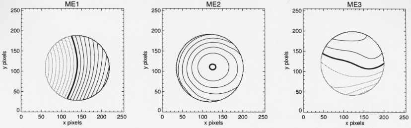Fig. 3. Relative gain maps (gain as percentage of the value at detector centre). Thick lines indicate a gain of 1.00. Contours are spaced by 0.01. Contours lower than 1.00 are in lighter shade

is 0.90 - 1.10 for ME1, 0.99 - 1.06 for ME2 and 0.96 - 1.03 for ME3, with a rms error 0.002 on almost all the field of view (excluding the ⁵⁶Fe calibration sources region where data were extrapolated).

4.3. Energy to channel conversion

Energy-to-channel conversion, energy resolution, and spectral profile of the MECS instrument have been determined from a detailed analysis of the calibration spectra. For each PANTER calibration line (see Table 3), on-axis and off-axis MU measurements have been analysed.

Energy spectra have been accumulated by selecting data in Burst Length in order to reject both double events (long BL) and events that convert in the scintillation region (short BL), as will be explained in Sect. 4.7.4. The relative gain maps (see Fig. 3) have been used to correct for the position gain dependence. Temporal gain dependence, mainly due to the temperature, have been taken into account by using the mean gain of the two 55 Fe inner calibration sources.

Fig. 4 shows the Cr line spectrum as detected by the ME2 unit as an example. Apart from the main peak, the spectrum shows several characteristics. In the low energy part are clearly present some features produced by the escape of fluorescence photons from the detector gas cell; they are present only for incident energies greater than 4.78 keV (the Xe L-edge). The phenomenon strictly depends on the geometry of the cell and on the gas filling pressure. In the case of the MECS, fluorescence photons mainly escape from the Be window and the escape fraction is expected to decrease when the energy increases, due to the greater penetration depth of the incident photon.

The bridge connecting escape and main peaks is due to the loss of a part of primary electrons for window attachment. In fact, in consequence of the primary interaction of the X-ray photon with the Xe atoms, an electron cloud is produced. This cloud diffuses toward the scintillation

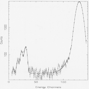Fig. 4. Energy spectrum of the Cr line (5.42 keV) with the fitting curve superimposed

region under the effect of the drift electric field. However, if the primary interaction takes place near the Be window, part of electrons is captured by the window itself, producing a smaller energy deposit (Inoue et al., 1978).

The spectra are fitted as a whole (see as example the continuous line in Fig. 4) by a function which is a sum of various components: a gaussian for the main peak, four gaussian for the escape peaks, and an exponential plus a constant to model the electron attachment phenomenon. For energies below 4.78 keV, the fitting model is simplified due to the absence of the escape peaks.

In some cases, as for the Ti spectrum shown in Fig. 5, there is clear evidence of a secondary, unresolved peak, the two components being the K_alpha and K_beta Ti lines; a better fit is then obtained by using two gaussian curves (the dotted curve in Fig. 5 represents the fit with a single gaussian, only).

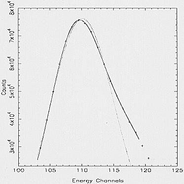Fig. 5. Energy spectrum of the Ti line (4.52 keV) of the central peak region. The dotted line refers to a single gaussian fit; the continuous line represents the double gaussian fit

In Table 4 the total escape fractions are reported. The experimental values are in good agreement with the prediction of a numerical model of the detector; no variation has been found as function of the incident photon position.

---

Table 4. Experimental total escape fraction

Line	Energy	Escape
	(keV)	(%)
Cr	5.42	2.23
Fe	6.41	1.84
Cu	8.06	1.42

---

Fig. 6 shows the results of the gain analysis for the detector unit ME2 (ME1 and ME3 units present a similar behaviour). The discontinuity at 4.78 keV (the jump in the detector gain) is caused by a decrease in the photonelectron conversion efficiency of the gas at the Xe L-edge (Santos et al., 1991, Dos Santos et al., 1993). This effect was also found in the EXOSAT, Tenma (White, 1985), and Spacelab GSPC detectors. The solid straight line in Fig. 6 corresponds to the best fit of the experimental points on each side of the edge (Mg, Al, Si, P, Ag and Ti lines for the left side; Cr, Fe and Cu lines for the right side).

Fig. 6. Gain vs. energy relationship for the ME2 detector unit. The discontinuity region due to the L-jump is zoomed in the insert

The fit procedure performed with the law

Gain =	A · E + B1	for E 4:78 keV
	A · E + B2	for E $>$ 4:78 keV

with Gain expressed in channel and E expressed in keV, gives the best A, B₁ and B₂ coefficients for each detector unit; the derived value of the L-jump discontinuity, averaged over the three units, is 110±15 eV, in good agreement with previous measurements (Lamb et al., 1987, Dos Santos et al., 1993).

4.4. Energy resolution

The spectral analysis allows to derive the energy resolution of the three MECS units for each PANTER calibration line.

The experimental values, in the form of Full Width Half-Maximum (FWHM), have been fitted by:

[(D E) / E] = A (6 / E)^½ (%)

where E is expressed in keV. The best fit values for the parameter A are 8.30(±0.08), 8.10(±0.08) and 7.68(±0.07) for ME1, ME2 and ME3 respectively, in agreement with the expectation for this kind of detector. In fact, the theoretical limit for the energy resolution of a GSPC is:

[D E / E] (% FWHM) = 2:35 (F / N)^½ x 100

where F is the Fano factor and N is the mean number of primary electrons produced by the X-ray photon. For the Xenon, typical value of the Fano factor is ~0.2. The mean energy to produce an electron-ion pair in Xenon is 22 eV. Using these values, the theoretical limit for the energy resolution is ~6.50% at 6 keV (Ramsey et al.,1994).

In the central region of the detector gas cell (10 mm radius) no position dependence of the energy resolution is pointed out within the experimental errors.

As an example, the ME1 spectral resolution versus energy is plotted in Fig. 7.

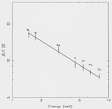Fig. 7. Spectral resolution vs. energy relationship for the ME1 detector unit

4.5. Image linearization

The position response of the detector is affected by some nonlinearities coming from three main contributions. The first most likely derives from spatial disuniformities in the PMT gain; the second one is due to a geometrical effect, i.e. different scintillation positions are seen by the PMT under different solid angles, leading to a variation in the light collection and then to an erroneous determination of the scintillation event position. These two effects are energy independent. The third contribution may be related to the distortion of the electric field near the Be window, due to a slight curvature of the window itself. This effect is more enhanced at low energy because of the shorter mean penetration depth of low energy photons (0.4 mm being the mean penetration depth of 1.5 keV photons with 1 atm of Xe) that produce a shift of the scintillation point with respect to the point in which the X-ray photo-absorption occurs.

In order to correct for these effects, the multipinhole measurements have been analysed; for each energy at least one measurement has been made and, in some cases, a scan has been performed, shifting the mask by steps usually of 1 mm or (sub)multiple, in order to have a fine coverage of the detector sensitive area with a grid of 1x1 mm. As a preliminary step, the detector electronic axes were verified to be aligned with the detector geometrical axes (determined by the strongback ribs) by using FF measurements at low energies, where the shadow produced by the window strongback is clearly visible. This allowed to correct for a slight rotation (£1^o ) between multipinhole mask and detector axes.

The barycentres (in pixels) of the spot images generated by the multipinhole mask, placed 1690 mm away from the detector, have been calculated through a bidimensional gaussian fit. Then, taking into account the real pitch of the holes as projected onto the Be window, a transformation law has been derived to convert the coordinates from pixels to millimetres. The transformation law that best fits the data is a third order polynomial, with a dependence on the energy only in the linear term.

X = A₃ [(1+ A₅) / E][K_x - A₁] + A₇[K_x - A₁]² + A₉[K_x - A₁]³

Y = A₄ [(1+ A₆) / E][K_y - A₂] + A₈[K_y - A₂]² + A₁₀[K_y - A₂]³

where K_x and K_y are the coordinates in pixels, E is the energy in keV, X and Y are the new coordinates (expressed in mm) and A_i are the best fit parameters.

The plate scale of three dectors is ~0.17 mm/pixel. A small anisotropy in the linear coefficients A 3 and A 4 is present between the coordinate axes: in particular, it is ~5% for ME1, while it is negligible ( 1%) for ME2 and ME3. Fig. 8 shows the result of the application of the above linearization formula on the Cu line data acquired with the multipinhole mask scan.

The transformation law reported here reconstructs the position of the holes with a rms error of 90 ^-6m in a central region of 6 mm radius, and of 120 ^-6m in the whole detector. These two values should be considered upper limits with respect to the actual values because they contain also the contribution of the mask hole position uncertainties. In the linearization procedure, the energy value E will be derived from the channel-to-energy conversion law. Due to the good MECS spectral resolution, this procedure will introduce a small additional uncertainty of ~10 ^-6m. A different approach, that is a correction of the geometrical distortions based on a XY plane correction map, is under evaluation.

4.6. Point spread function

The Point Spread Function (PSF) of the MECS is the convolution of the MU PSF and the detector PSF. The

Fig. 8. Multipinhole data of the Cu line for the ME3 detector unit. The position (0,0) refers to the center of the detector. Each pin connects the actual hole (point of the pin) with the measured position (pin's head). a) analysis made with a constant plate scale factor (0.17 mm/pixels); b) analysis performed by using the third order linearization polynomial

precision with which an X-ray event is localized in the detector is essentially determined by the number of electrons which are liberated by the interaction of the photon with the Xenon gas contained in the detector cell. Thus the detector PSF is expected to be a gaussian with oe / E =2 .

The multipinhole data acquisitions have been used to measure the detector PSF. We find the data to be in good agreement with theoretical predictions for energies E4 keV while, for E$>$4 keV, the oe appears to be larger than expected. The disagreement between data and model is due to the fact that, at high energies, the size of the PSF becomes comparable to the size of the holes, making the pinhole approximation as a point-like source no longer valid. In principle, the oe of the detector PSF, at high energies, could be recovered by convolving the emission from a hole of finite size with a gaussian, and then by fitting this convolution to the experimental data. In practice, it can be more conveniently derived from the FF data, by measuring the radial distribution of photons in proximity of the detector unit edge (a preliminary analysis confirms the E PSF. An analysis of the off-axis PSF is currently under way, and it will be reported elsewhere. Preliminary results indicate that, for off-axis angles 10 arcmin, the departure of PSF shape from radial symmetry is relatively small, thus allowing us to apply the radial description of the on-axis PSF hereafter outlined. For off-axis angles $>$10 arcmin, i.e. outside the strongback region, an azimuthal dependence of the PSF becomes apparent.

In order to obtain corrected on-axis PSF images of the MECS system we have:

- accumulated images from the MU on-axis and FF data acquisitions at each of the PANTER calibration lines (as listed in Table 3, but the Cu L_alpha line);

- corrected the images for the spatial dependence of the gain (cfr. Sect. 4.2);

- converted the images from raw pixels to linearized pixels (cfr. Sect. 4.5);

- applied BL and energy selections in order to reject contaminating background events;

- divided each PSF image by the FF image taken at the same energy.

Finally we have accumulated radial profiles from the corrected PSF images. The fit of the radial profiles have been performed with a PSF model which is the sum of two components: a gaussian, G(r), and a generalized lorentzian, L(r):

G(r) = c_g exp[(-r²) / (2 s²)]

L(r) = c_l[1 + (r / r_l)²]^-m

where r is the distance from the peak of the emmission and c_g, c_l, s, r_l, and m are the parameters of the model. As an example, in Fig. 9 the fit to Al line data is shown. As can be seen, the very high statistics (~500.000 events in each MU on-axis data acquisition) allows us to measure the PSF up to 20 arcmin corresponding to 60 pixels.

Fig. 9. Differential PSF at 1.49 keV (Al line) for the ME3 detector unit

By imposing that the integral of the PSF over the entire plane be equal to unity,

2 p ò PSF(r)r dr = 1

we have reduced the number of independent parameters to four: s, r_l, m, and R, where R = (c_g / c_l) . The dependence of these four parameters on energy has been reproduced through simple algebraic functions. As an example, the fit of the values derived at the PANTER calibration lines for the parameter R is shown in Fig. 10.

The complete analytical expression for the on-axis PSF is:

PSF(r,E) = 1 / 2p[R(E)s2(E) + (r2l(E)) / 2(m(E) -1)] x

{ R(E) exp( + [ 1 + ( r / (rl(E)) ) 2 ]-m(E)

where R(E), s(E), r_l, and m(E) are algebraic functions of E. Since both G(r) and L(r) can be analytically integrated in r dr, the PSF equation can be used to derive a mathematical expression for the Integral Point Spread Function:

IPSF(r) = 2p ò PSF(r) r dr

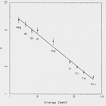Fig. 10. The R parameter, defined as cg =c l , as a function of energy for the ME3 detector unit

This equation has been used to evaluate the 50% and 80% Power Radius (PR) at three different energies for the ME3 unit; the derived values are reported in Table 1 (ME1 and ME2 units give PR values very close to the ME3 ones).

4.7. Effective area

The total MECS effective area, A_e (E,theta), results from the MU effective area (A_MU), reduced by some transmission coefficients related to the plasma protection grid (T_f1), the plasma/UV filters (T_f2), the Be window (T_w), and to the detector efficiency (P_a); a further reduction coefficient (BL_s) due to the Burst Length selection must be also considered:

A_e(E,theta) = A_MU,infi(E,theta)·T_f1 · T_f2(E)· T_w(E)·P_a(E)·BL_s(E)

Fig. 11 shows the MECS (3 units) effective collecting area as function of energy for different off-axis angles. All the effective area components will be described in the following sections. It is important to point out that, during the on-ground calibration, measurements of the absolute efficiency have been done only for the optics. The effects of the other components are evaluated mainly by simulations.

4.7.1. Mirror efficiency and vignetting

The MU effective area is given by:

K·A_det · N_MU / N_FF · E_FF / E_MU · T_FF / T_MU

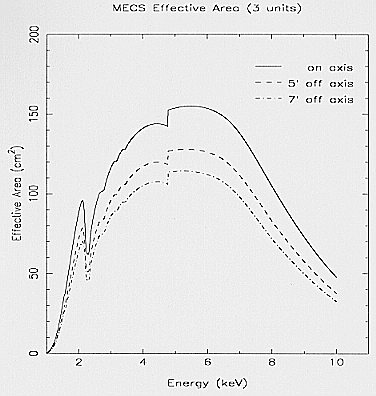Fig. 11. The MECS effective collecting area as function of energy for different off-axis angles

where N_MU and N_FF are the number of counts detected during a Mirror Unit and a Flat Field measurements respectively, T_MU and T_FF are the exposure times corrected for the instrumental dead time,E_MU and E_FF indicate the detector efficiency for MU and FF measurements respectively, A det is the geometrical area of the detector, and K is a correction factor taking in account the different flux, on the detector and on the Mirror Unit, due to their different distance from the X-ray beam source.

E_FF is in general different from E_MU . In fact, during a FF measurement, the X-ray flux is spread on the entire Be window and partially absorbed by the strongback structure while, during a MU measurement, the X-ray flux is well concentrated in a small region of the window due to the optics spread function, and only for particular offaxis angles it is absorbed by the strongback structure. The difference between the two values E_MU and E_FF is significant below a few keV while it becomes negligible above 4 keV.

N_MU and N_FF were computed by accumulating events in selected energy intervals. The detector energy gain was corrected for the position distortion by using the correction maps (see Sect. 4.2), and for the time variation by using the gain of the inner 55 Fe calibration sources.

The instrumental background, measured in a long detector exposure with the X-ray beam switched off, was subtracted from the accumulated events. Furthermore, two regions of 3 mm radius around the inner ⁵⁵Fe calibration sources were excluded from the accumulation process.

For each PANTER calibration line (see Table 3) we obtained a set of effective area values corresponding to the different off-axis positions. Each set at energy E i was fitted by the function:

A(E_i,theta) = A₁(E_i)·V(E_i,theta)

where

V (E_i,theta) = [1 / (1 + A₂(E_i) · theta^A₃(E_i))]

is a vignetting factor with

theta = P [(X_j - X_j)² + (Y_j - Y_j)²]^½

where X_j and Y_j are the baricenter coordinates (mm) of the spot image during a MU measurement at off-axis theta, X_o and Y_o are the on-axis focal plane coordinates, and P is the MECS plate scale factor. X_o, Y_o, A₁(E_i), A₂(E_i), and A₃(E_i) are free parameters of the fitting procedure. A₁(E_i), the maximum of the function, is the MU on-axis effective area.

Fig. 12 shows the on-axis optics effective area for each of the three MECS mirror units. The theoretical effective area has been computed by considering the optics coned geometry and the Au reflection coefficient (Henke et al., 1993 ). The agreement between theoretical and experimental results has been reached by multiplying the theoretical value with a second order polynomial of energy. The best polynomial parameters are obtained by fitting experimental data; the result of the fitting, A(E,0), are reported in Fig. 12 as a continuous line, while the diamond markers represent the A₁(E_i) values. The general equation becomes:

A(E,theta) = A(E,0)·V(E,0)

For each energy E_i-1 < E < E_i, the vignetting factor V(E,thete) is derived by interpolation of the experimental values V(E_i-1,theta) and V(E_i,theta)

The results shown in Fig. 12 refer to the case of an emitting source located at 130 m from the optics (PANTER configuration). The finite distance of the source produces a loss of effective area compared to the case in which the emitting source is located at infinite distance. In fact, for finite distance, the beam is divergent, and a small but not negligible fraction of the radiation is imaged in a region around the focus. This region appears as a large radius annulus in the case of on-axis source direction (theta = 0^o ), and it assumes a more complicated shape for large theta values. The intensity of the loss radiation is function of energy, too; being each mirror at different slope, their contribution to the finite distance radiation loss are different: high energy photons (E $>$6 keV) are reflected mainly by the inner optics, while low energy photons by the entire optics system.

To obtain the correct A_MU,infi (E,theta) starting from the A(E,theta) values, we simulated, by means of a ray-tracing software, both the infinity case (parallel beam) and the PANTER case (divergent beam) for several values of E

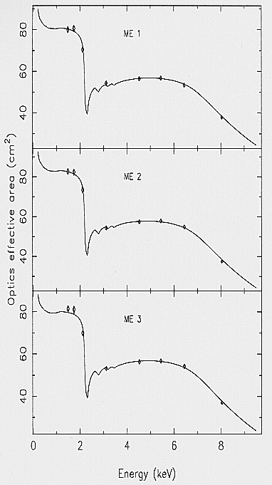Fig. 12. On-axis optics effective area vs. energy for each MECS unit. The diamond markers correspond to the A1(E i ) values (see text). The continuous lines, A(E,0), represent the theoretical expectation multiplied by a second order polynomial

and theta. The optics geometry was followed in all its details by the traced rays, and only the radiation reaching the focal plane whithin a circle corresponding to the Be window, was taken into account for the computation of the effective area. Two different sets of values have been produced, namely A_infi(E,theta) and A₁₃₀(E,theta). Finally, the relation between A_MU,infi and A(E,theta) can be written as:

A_MU,infi(E,theta) = [A(E,theta)·A_infi(E,theta)] / [A₁₃₀(E,theta)]

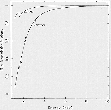Fig. 13. LEXAN and KAPTON filter transmission efficiency vs. energy. Circles indicate measured values (Jager, 1996)

4.7.2. UV/ions shield windows

In order to avoid that the plasma particles crossing the MU can accelerate towards the Be window set at -8 kV, a plasma protection grid is mounted below the optics system. The grid in Au-coated tungsten is kept at +28 V, shielding the Be window electric field. This grid causes a loss of effective area of 8% (T_f1 = 0.92), independent on the energy. Furthermore, to be sure that any high velocity plasma component overcoming the grid shielding doesn't impinge on the Be window, plasma filters have been placed in front of them. The filters stop also UV light photons that could extract electrons from the Be window; these electrons, accelerated by the Be window electric field towards the MECS Carbon fiber walls, should produce a background increase due to the electron bremsstrahlung emission.

The first solution adopted for plasma/UV damage protection was the use of thin Polyimide filters, as in the LECS case (Parmar et al., this volume), and the MECS on-ground PANTER calibrations were performed with this kind of filter. Unfortunately, after vibration test, one of the Polyimide filters was found to be destroyed. Now, in the flight configuration, ME2 and ME3 units are both protected by a LEXAN filter 0.6 ^-6m thick, aluminium plated by two layers of 0.035 ^-6m, each; for precautionary reason, the third unit, ME1, is protected by a 7.6 ^-6m thick KAPTON filter, aluminium plated by two layers of 0.1 ^-6m, each. Fig. 13 shows the transmission efficiency T_f2 for the two filters.

4.7.3. Beryllium transmission

No measurements of the Be window transmission efficiency Tw were performed during the MECS on-ground calibrations; anyway, this efficiency can be computed analytically by:

T_w = exp(-mu(E)·x)

where mu(E) is the absorption coefficient of the material at the energy E, and x is the thickness. Fig. 14 shows the transmission effciency for a layer of 50^-6m (window thickness) and for a layer of 600 ^-6m (window plus strongback thickness), representing the two different regions of the detector window, as shown in Fig. 2 (verification of strongback thickness from FF measurements is in progress).

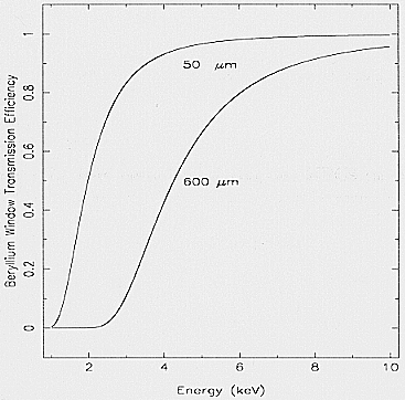Fig. 14. Beryllium transmission efficiency vs. energy for two different thickness values

4.7.4. Detector efficiency and burst length selection

The gas cell absorption probability P_a is:

P_a = 1 - exp(-mu_Xe(E)·D)

where mu_Xe is the Xe absorption coefficient for the energy E, and D is the size of the absorption region. Fig. 15 shows the gas cell efficiency obtained with D equal to the drift region depth; events that convert in the scintillation region are rejected to improve the energy resolution.

In Fig. 16 the BL versus energy pseudo-image (contour plot) for the Cu line spectrum is shown. The spot ''a'' refers to events which convert in the drift region with a single electron cloud giving correct PHA and BL values;

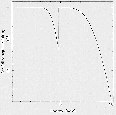Fig. 15. Gas cell absorption efficiency for the drift region vs. energy

this kind of events make up more than 90% of the total events. The spot ''b'' refers to the residual events; these events present a single electron cloud too, but an incorrect PHA value (see Sect. 4.3 for further details). The bridge between ''a'' and ''b'' is mainly due to events that, interacting with the Xenon near the Be window, loose part of the electrons for attachment to that window. This phenomenon is seen as a low energy tail in the line spectra (as already explained in Sect. 4.3). The tail ''c'' is due to events which are absorbed in the scintillation region producing a reduced amount of UV light (and a shorter BL), resulting in an incorrect PHA value due to the shorter path in that region. These events, in the case of the Cu line (8.06 keV), are 4.5% of the total number of events; for lower energies, this fraction decreases due to a shorter penetration depth (see Fig. 15). The jet ''d'' is due to some of double events, i.e. to events with the fluorescence photons re-absorbed inside the gas cell but at a different position from the primary conversion. This effect produces correct PHA value but a higher BL value due to the sum of the two scintillation bursts; the position detected for these events (2.4% of the total number) should be incorrect being the weighted average of the two interactions. The rejection of ''c'' and ''d'' events is performed by using a suitable BL selection. Such a kind of picture is typical of energies greater than 4.78 keV (the Xe L-edge); for lower energies, the regions ''b'' and ''d'' disappear while the ''c'' region becomes negligible. A BL_s (E) function has been derived to introduce the effect of the selection in the MECS total effective area (A_e(E,theta)) computation.

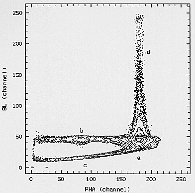Fig. 16. Burst Length vs. energy pseudo-image for the Cu line

4.8. Background counting rate

Two components will be present in flight:

- the induced particles, and

- the diffuse X-ray, due essentially to the extragalactic component. The galactic component, mainly at low energies, is not detected because of the Be window transparency (less than 5% below 1.0 keV).

Environmental charged particles, interacting with the gas in the detector, loose their energy producing electron clouds. The dimension of the clouds is generally bigger than the one due to X-ray photons of equivalent energy, because of the longer path the particle covers before being stopped. The Burst Length, proportional to the cloud dimension, can then be used to discriminate genuine photons from charge induced events.

Measurements of the environmental background have been performed during the PANTER and ESTEC calibration campaigns. The longest background accumulation, relative to the ME1 unit, has a duration of ~=9 hours. Data used for the evaluation of the residual background have been opportunely selected in BL and in position. Fig. 17 shows the image of the residual background after the BL selection applied during the data analysis. The circle indicates the region used for the analysis: the outer region is not considered in order to exclude both the two spots produced from the inner ⁵⁵Fe calibration sources and the high density outer ring; this ring is due to events converting in the outer part of the detector (outside Be window diameter) and compressed towards the internal region by the readout system.

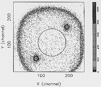Fig. 17. Environmental background image. The circle delimits the region for which are valid the data reported in Table 5

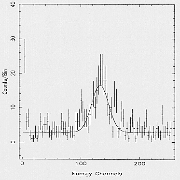Fig. 18. Residual background spectrum within the circle as in Fig. 17

The spectrum of the selected events is shown in Fig. 18. The spectrum was fitted with a constant plus a gaussian; the results of the fit are shown in Table 5. A line-type feature is evident in the central part of the spectrum. Possible explanations of this feature are: a) fluorescence by detector material (as the NiCo ring in Fig. 1); b) re-absorption, far from the primary interaction point, of fluorescence emitted from the 55 Fe calibration sources; c) combination of the two above effects. The background is in any case very low and the statistics collected during the on-ground cali bration does not allow a conclusive analysis of the nature of the line. A deeper analysis of the detector background will be performed with the in-flight data.

---

Table 5. Background counting rate: results of the fit

Parameter	Value
Flux of the constant	(4.95±0.59) 10-4 cts/cm2/s/keV
Flux of the line	(13.5±1.3) 10-4 cts/cm2/s
Energy of the line	6.07±0.13 keV
Line width	~= 8.2 % (compatible with the detector resolution)

---

Estimation of the in-flight residual flux of charged particle background from previously flown (EXOSAT) and currently operating (ASCA) Gas Scintillation Proportional Counters brings to a conservative value of 2·10^-3 cts/cm²/sec keV in the 2 - 10 keV band.

Evaluation of the expected count rate from the extragaltic component of the diffuse background has been made by simulating photons coming from off-axis up to 1^o with uniform angular distribution. The spectrum used in the simulation is a power law of spectral index 1.5 corrected, at low energy, for the galactic absorption from a column of 3·10²⁰/cm². The obtained count rate is 1.3·10^-3/cm²/sec/keV, where cm² is referred to the considered detector area.

Acknowedgements

We wish to thank L. Scarsi for the effort he spent in supporting BeppoSAX mission, R.C. Butler for his tenacious interest in the scientific instruments, O. Citterio for the work in developing the technology and the testing methods of the Mirror Units, G. Manzo for the original contribution to the design and development of the ME detector. G. Ferrandi, E. Mattaini, and E. Santambrogio, from IFCTR Institute, provided the mechanical calibration support equipment. We thank H. Brauninger and W. Burkert for the support to the calibration activity at the PANTER facility. L. Casoli, M. Confalonieri, P. Dalla Ricca, T. Motta, A. Prestigiacomo, G. Rimoldi, A. Sada, P. Sarra, and L. Vierbi, from Laben industry, sub-contractors for the MECS instrument, assured the management of the detectors and of the data acquisition system during the calibration campaigns. S.Molendi acknowledges useful discussions with H. Ebeling on PSF models. We wish thank K. Ebisawa for the useful suggestions to improve this paper. All the activities of the Scientific Institutes have been financially supported by the Italian Space Agency (ASI) in the framework of the BeppoSAX mission.

References

• Boella, G. et al. 1995, Proc. SPIE Conference, San Diego, CA, USA, Paper n. 2517-14
• Boella, G. et al. 1996, this volume
• Butler, C., Scarsi, L. 1990, SPIE 1344, 46
• Citterio, O. et al. 1985, SPIE 597, 102
• Citterio, O. et al. 1988, Appl. Opt. 27, 1470
• Conti, G. et al. 1993, SPIE 2011, 118
• Conti, G. et al. 1994, SPIE 2279, 101
• Dos Santos, J.M.F., Conde, C.A.N., Bento, A.C.S.S.M. 1993, NIM A324, 611
• Henke, B.L., Gullikson, E.M., Davis, J.C. 1993, Atomic Data and Nuclear Data Tables 54, 2
• Inoue, H. et al. 1978, NIM-PR 157, 295
• Jager, R. 1996, private communication
• Lamb, P. et al. 1987, Astrophysics and Space Science 136, 369
• Molendi, S. et al. 1995, Proc. Int. Conf. on X-Ray Astronomy and Astrophysics, W¨urzburg, Germany, in press
• Parmar, A.N. et al. 1996, this volume
• Ramsey, B.D. et al. 1994, Space Science Rev. 69, 139
• Santos, F.P. et al. 1991, NIM A307, 347
• White, N.E. 1985, EXOSAT Express 11, 51

---