Table of Contents
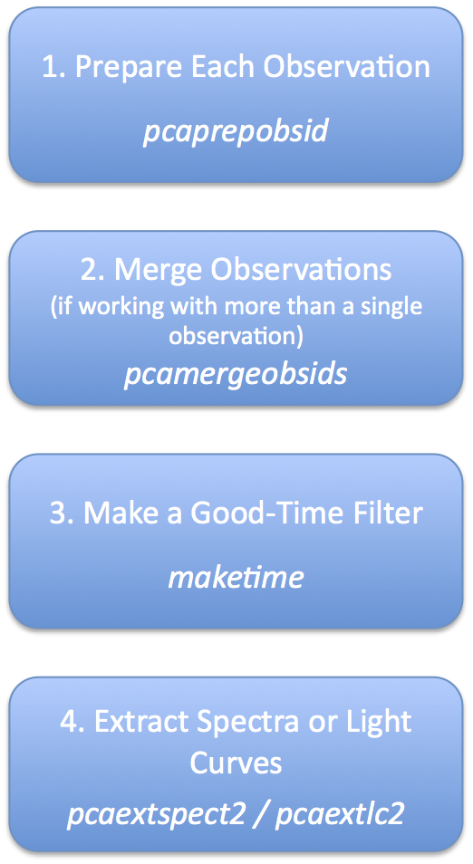
IntroductionAnalyzing RXTE data can appear to be a difficult process but it does not need to be. This document describes a set of tools that make processing RXTE PCA data quite straightforward, and removes a lot of the guesswork. This document provides an overview of how to analyze RXTE Standard2 data, which is a data mode active for every observation in the RXTE archive. Standard2 data has 16 second temporal resolution and good energy resolution. For spectral analysis on time scales longer than 16 seconds, Standard2 data is the best choice for data analysis. The PCA instrument team has developed a set of tools and practices that will automatically filter the data and provide a high quality output. Note that this document and software covers Standard2 mode data only (files beginning with FS4a_*). It does not cover Standard1 mode (FS46_*) or other data taken in Binned data modes. Also, it does not cover data taken in Event mode. If you or your colleagues have developed your own scripts to analyze RXTE data, then you do not need to stop using your scripts. These tools are a layer on top of existing RXTE software. It is hoped however that these tools provide a reference for users to be sure they are deriving high quality results. These tools are part of the standard HEASoft / FTOOLS software release. If you have a recent version of this software (published after June 2013, then you have all of these tools). You will also need a recent version of the RXTE Calibration database (CALDB). Although this process is simplified, it is not simple. All of the power of the original FTOOLS analysis is available to the user. The new simplified tools remove most of the extraneous choices, but the scientific user still has the choice of setting most of the lesser-used options if they wish. OverviewRXTE data, as it comes from the archive, is in a "mostly raw" state. At the time of RXTE's design, the philosophy was to store the raw data with as little manipulation or processing as possible, and let the user process the data later with up to date software and calibration. Thus, it is necessary for most users to run a series of data processing steps to produce usable science products. The RXTE archive does create standard products which are usable for "quick look" types of activities. Also, if you are interested in context information about a particular target, be sure to consult the RXTE mission long light curves. Generally speaking, the standard products are produced on an observation-by-observation basis with standard filtering and reasonable default values for settings. If you want to produce different types of products or use different filtering, then you will need to perform your own analysis. Figure 1 shows an overview of the analysis process with these recommended tools. This section provides an overview of the overall process, and later sections provide more detailed information. The analysis is divided into four basic steps.
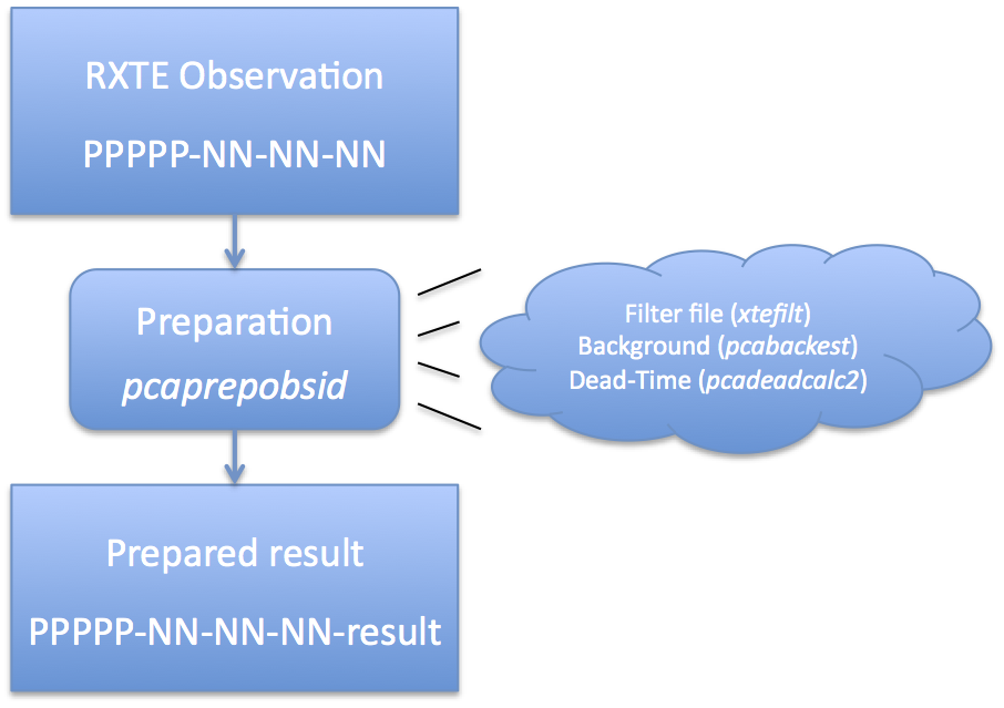
Now let us look at these steps in more detail. Preparation of PCA DataAs mentioned above, RXTE archive data comes in a very raw form. It is necessary to run a set of standard tools which prepares this data for analysis. The task 'pcaprepobsid' is a standard FTOOL which accomplishes this task. See Figure 2 for an overview of this process, and you can read about it in more detail on the PCA data preparation page. As Figure 2 indicates, each observation must be processed once by 'pcaprepobsid'. The input of 'pcaprepobsid' is a single observation directory, which should have the format delivered by the RXTE archive. For example, a single observation directory will have name 93046-01-02-00, where 93046 is the proposal number, and the later numbers indicate target and visit numbers. The directory contains a single FMI file, as well as pca/, acs/ and hexte/ subdirectories. You cannot use 'pcaprepobsid' on a full proposal-level directory, but must run it once for each observation within a proposal subdirectory. 'pcaprepobsid' runs some standard tools that long-time RXTE users will recognize, and some that they may not. It runs 'xtefilt' to create a filter file. It also runs the task 'pcabackest' on each Standard2 file to create a background estimate. It runs the task 'pcadeadcalc2' to calculate dead-time quantities for each Standard2 file. The output of 'pcaprepobsid' is a new subdirectory which contains several output files. More information about the output directory can be found on the detailed PCA data preparation page. To run 'pcaprepobid', you can run it on the command line, and it will prompt you for inputs: csh> pcaprepobsid > Name of input observation ID directory [93067-01-42-01] 93067-01-42-01 > Name of output results directory [93067-01-42-01-result] 93067-01-42-01-result > Running pcaprepobsid v1.0 > ---------------------------------------- > 93067-01-42-01 2008-04-14T21:50:39 2008-04-14T22:06:17 > FILT: 93067-01-42-01-resultlr 9/FP_1adf146f-1adf1819.xfl > STD2: 93067-01-42-01/pca/FS4a_1adf146f-1adf1819.gz In this case, you were prompted for the observation directory (93067-01-42-01) and the output prepared results directory (93067-01-42-01-result). The remaining text is the output of the task, which shows that it is making a FILTer file and making Standard2 background and deadtime calculations. Like all HEASoft tasks, you can also run 'pcaprepobsid' in non-interactive mode, a convention we will adopt for the remainder of this document. In that case, all of the inputs need to be specified on the command line. For example, the same processing as above can be achieved with, pcaprepobsid indir="93067-01-42-01" outdir="93067-01-42-01-result" Until the new PCA background model is in CALDB, you will need to specify the background model manually on the command line, like this,
  pcaprepobsid indir="93067-01-42-01" outdir="93067-01-42-01-result" \
    modelfile="/path/to/pca_bkgd_cmvle_eMv20111129.mdl.gz"
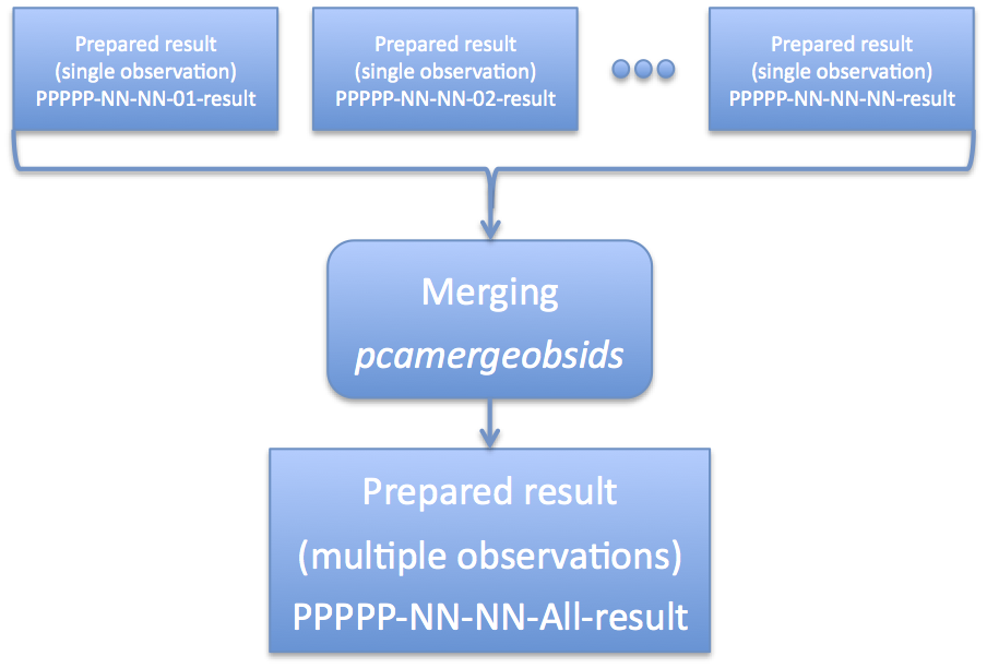
After running 'pcaprepobsid', you should now have an output directory -- 93067-01-42-01-result in this example -- which you will use for further processing. Run this process once for each observation of interest. If you are interested in combining multiple observations for analysis, then read on to learn about merging observations. You can read more about preparing your observations, including details about the contents of the output directory, how easily run the task for multiple observations, and other special settings at this PCA data preparation detail page. Optional Step: Merge Multiple ObservationsAs mentioned above, it is quite often that a single scientifically interesting observation is broken into multiple RXTE observational data sets. In some cases, this may be at the request of the observer (for example, multiple monitoring observations), but in other cases a long RXTE observation must be broken into several parts for practical reasons. However, at the scientific analysis stage, one will often desire to combine multiple observation data sets into a single logical data set. This is not difficult, and the RXTE software handles multiple files straightforwardly. Because there are several sets of files to keep track of -- source files, background files, filter files, etc -- it would be nice to have way to automate this process. Enter the task 'pcamergeobsids'. Figure 3 gives an overview of what this task does. As indicated by Figure 3, 'pcamergeobsids' accepts one or more input prepared results, and produces a single output prepared result which combines all of the inputs. If you have investigated the contents of a prepared result, then you know that it contains various processed Standard2 files and background files, as well as filter files and list files. What 'pcamergeobsids' does is combine each of those files in a self consistent way so that it appears that multiple observations are one single meta-observation. You run the task 'pcamergeobsids' in the following way, # Make a file which lists all prepared result directories # NOTE: tailor this to the names of your result directories! ls -d 93067*-result > 93067-all.lis pcamergeobsids indir=@93067-all.lis outdir=93067-all-result The 'indir' parameter accepts a list of input directories, which should be results prepared by 'pcaprepobsid'. It is also possible to merge the output of 'pcamergeobsids' with other data sets! The 'outdir' parameter gives the name of the new prepared results. The "@filename.lis" pattern is a common one within HEASoft. It indicates that filename.lis is a file that a list of multiple files. Using the standard Unix wildcard matching, it's possible to create such a file. In the example above, the pattern "93067*-result" would match all directories that have been produced by the task 'pcaprepobsid' beginning with that obsid name. Note that you want to list the names of the directories and not the contents. This is why the '-d' option to 'ls' is so very important. By default the task 'pcamergeobsids' does not copy the large data files, but links to them instead. Please see the detail PCA data preparation page for more information. Make a Good Time FilterOnce you have created a set of prepared results, either from a single observation or the result of merging multiple observations, you are ready to start performing filtering. At a basic level, filtering removes bad data and keeps good data for scientific analysis. But which is bad and which is good? This is a stage where more scientific judgement enters into the picture as well. There are some kinds of filtering that all users should do. Every user should screen data to remove data when the target is below the earth horizon (ELV cut), and or when RXTE is not pointed at the desired target, or when PCU detectors are off. This may seem obvious, but because RXTE typically includes all data taken, even data during slew to the target or observation setup, there will be times in the data set when no scientific data are present. Thus basic screening criteria are needed for all users. There may be other, more interesting scientific screening criteria that might be applied as well. For example, do you only want to include data when an eclipsing source is in eclipse? Or when a black hole candidate has a high count rate? In those cases, you need to create a more finely nuanced set of screening criteria. Also, while you only "prepare" your observation data once with 'pcaprepobsid', you can create many different good time filters based on different filtering strategies. To learn more about screening criteria, see the screening detail page. The important thing to know is that once filtering has been done, this information is encoded in a file known as a Good Time Interval file, or GTI file for short. This file contains a list of starts and stops of filtered good intervals. In this overview, we will show how to make a single GTI file with basic screening criteria using 'maketime' You create a GTI file by passing screening criteria to the task called 'maketime'. The task 'maketime' is a standard HEASoft task which is used by many missions, including RXTE. Here is how you would call maketime in Unix csh/tcsh shell language:
  # Basic filtering expression.
  # NOTE: you may need to tailor it for your needs!
  set expr="(ELV > 4) && (OFFSET < 0.1) && (NUM_PCU_ON > 0) && .NOT. ISNULL(ELV) && (NUM_PCU_ON < 6)"

  set filtfile=`cat 93067-all-result/FP_xtefilt.lis`

  maketime infile=$filtfile outfile=93067-all-basic.gti expr="$expr" \
     value=VALUE time=TIME prefr=0.5 postfr=0.5 compact=NO clobber=YES
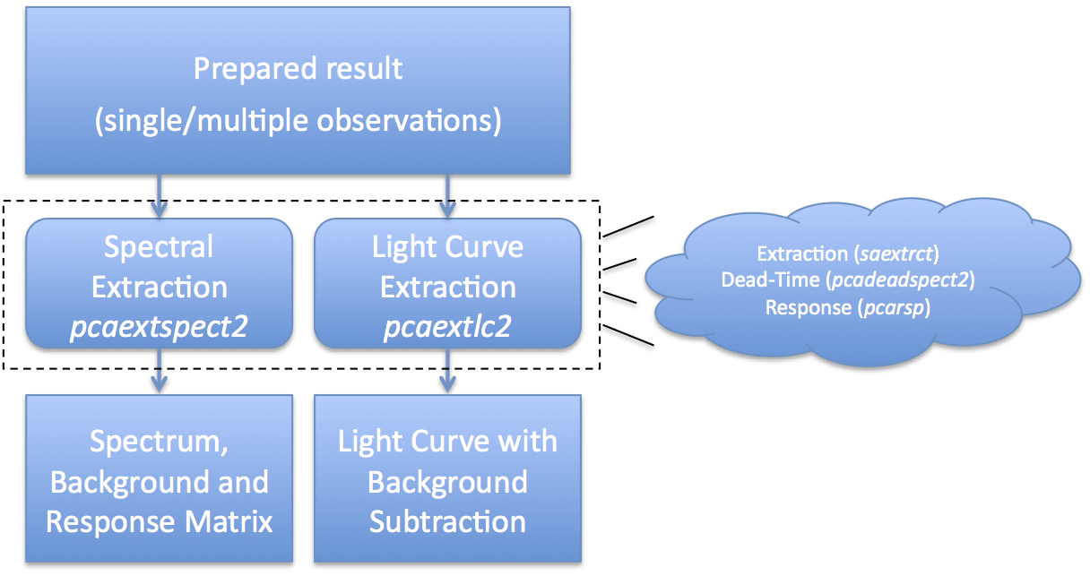
The task 'maketime' accepts as input the filter file for your observation data set, which is set here to the file pointed to by 93067-all/FP_xtefilt.lis (based on the example in the previous section). The output file will be a GTI file named 93067-all-basic.gti. The 'expr' parameter is the filtering expression itself. There are some other rote parameters that are needed for RXTE. What does this expression do? The expression "ELV > 4" means the target must be at least 4 degrees above the earth's limb (horizon). The expression "OFFSET < 0.1" means that the target must be within 0.1 degrees (6 arcmin) from the satellite pointing direction. The expression "NUM_PCU_ON > 0" ensures at least one PCU is enabled. The other filtering criteria are basic data quality checks. NOTE: this is only a very basic set of screening criteria. The screening detail page discusses in more detail other recommended criteria, especially if you are observing a faint target or have offset pointing. Extract Spectra or Light CurvesAt this point, you are at the step where you extract scientific products. The products we will discuss here are Standard2 spectra, obtained with the task 'pcaextspect2', and light curves, obtained with the task 'pcaextlc2'. These tasks are very similar, and differ only in the details peculiar to spectra or light curves. Figure 4 gives an overview of the extraction process. What Figure 4 shows is that you start with a set of prepared results, either from a single observation or the result of merging multiple observations. You run the task 'pcaextspect2' to obtain spectra and associated metadata, also known as PHA and RSP files; and 'pcaextlc2' to obtain light curves, also known as LC files. Internally, these extractors use the well-known standard tools like 'saextrct' for extraction and 'pcarsp' for response generation. For spectra, it is expected that you will extract both a source spectrum and a background spectrum. Every RXTE PCA observation has an associated background, and you must include background in your subsequent analysis. By default, both spectra are dead-time corrected. Also by default, each spectrum should have an associated PCA response matrix which provides information about the spectral sensitivity during your particular set of observations. You should not use a generic response matrix. For light curves, it is expected that you will be interested in both the source rate and background rate. By default, extracted light curves are background-subtracted and dead-time corrected. Here is an example to extract a spectrum:
  pcaextspect2 \
    src_infile=@93067-all-result/FP_dtstd2.lis \
    bkg_infile=@93067-all-result/FP_dtbkg2.lis \
    src_phafile=93067-all_src.pha bkg_phafile=93067-all_bkg.pha \
    gtiandfile=93067-all-basic.gti \
    filtfile=@93067-all-result/FP_xtefilt.lis \
    respfile=93067-all.rsp \
    pculist=ALL layerlist=ALL
This is a long command line which contains many parameter settings! The key thing is that the source and background input files ('src_infile' and 'bkg_infile') are taken from your prepared results with dead-time quantities computed. The output spectra ('src_phafile' and 'bkg_phafile') will be named 93067-all_src.pha and 93067-all_bkg.pha. The 'gtiandfile' parameter is the name of the good time interval file we created in the previous step. The 'filtfile' gives the name of the filter file associated with our prepared data, and 'respfile' tells the name of the output response matrix file. Finally the 'pculist' and 'layerlist' parameters tell the task that we want all good detectors and all good layers. Note that it is safe to specify pculist=ALL even if some PCUs are off or a high voltage breakdown occurred. The task is smart enough to tally only the live time of the enabled good detectors, and exclude the bad detectors. Here is an example to extract a light curve:
  pcaextlc2 \
    src_infile=@93067-all-result/FP_dtstd2.lis \
    bkg_infile=@93067-all-result/FP_dtbkg2.lis \
    outfile=93067-all.lc \
    gtiandfile=93067-all-basic.gti \
    pculist=ALL layerlist=ALL binsz=16
This command line is shorter, but many of the parameters should look familiar. The 'src_infile' and 'bkg_infile' parameters are the same, as are the 'gtiandfile' 'pculist' and 'layerlist' parameters. The 'outfile' is the name of the output light curve file. The new parameter 'binsz' gives the light curve time bin size in seconds, which must be a multiple of 16 seconds for Standard2 data. You may wish to choose different channel (energy) ranges, on your way to computing hardness ratios. In that case, you should investigate the 'chmin' and 'chmax' parameters. To understand more about extracting spectra and light curves, please see the PCA Standard2 extraction detail page. Where to Go from HereFrom here you can begin your scientific analysis in earnest. For spectra, the next stop is typically fitting your spectrum within the XSPEC fitting environment. For light curves, there are multiple possible next steps, including plotting (with the task 'fplot' or the viewer 'fv'); making light curves in multiple energy bands and creating hardness ratios; performing Fourier power spectral analysis with 'powspec'; and so on.
If you have a question about RXTE, please send email to one of our help desks.
|


- RXTE Project Scientist: Tod Strohmayer
- NASA Official: Rob Petre
- Web Curator: J.D. Myers
- Last Modified: 3-Sep-2020