|
Next: Simultaneous Fitting Up: Walks through XSPEC Previous: Brief Discussion of XSPEC
Fitting Models to Data: An Old Example from EXOSATOur first example uses very old data which is much simpler than more modern observations and so can be used to better illustrate the basics of XSPEC analysis. The sample files are found at https://heasarc.gsfc.nasa.gov/docs/xanadu/xspec/walkthrough.tar.gz. The 6s X-ray pulsar 1E1048.1-5937 was observed by EXOSAT in June 1985 for 20 ks. In this example, we'll conduct a general investigation of the spectrum from the Medium Energy (ME) instrument, i.e. follow the same sort of steps as the original investigators (Seward, Charles & Smale, 1986). The ME spectrum and corresponding response matrix were obtained from the HEASARC On-line service. Once installed, XSPEC is invoked by typing
%xspec as in this example:
%xspec

		XSPEC version: 12.12.1
	Build Date/Time: Mon Feb  7 15:09:57 2022

XSPEC12>data s54405.pha

1 spectrum  in use

Spectral Data File: s54405.pha  Spectrum 1
Net count rate (cts/s) for Spectrum:1  3.783e+00 +/- 1.367e-01
 Assigned to Data Group 1 and Plot Group 1
  Noticed Channels:  1-125
  Telescope: EXOSAT Instrument: ME  Channel Type: PHA
  Exposure Time: 2.358e+04 sec
 Using fit statistic: chi
 Using Response (RMF) File            s54405.rsp for Source 1
The data command tells the program to read the data as well as the response file that is named in the header of the data file. In general, XSPEC commands can be truncated, provided they remain unambiguous. Since the default extension of a data file is .pha, and the abbreviation of data to the first two letters is unambiguous, the above command can be abbreviated to da s54405, if desired. To obtain help on the data command, or on any other command, type help command followed by the name of the command. One of the first things most users will want to do at this stage – even before fitting models – is to look at their data. The plotting device should be set first, with the command cpd (change plotting device). Here, we use the pgplot X-Window server, /xs.
XSPEC12> cpd /xs There are more than 50 different things that can be plotted, all related in some way to the data, the model, the fit and the instrument. To see them, type:
XSPEC12> plot ?
plot data/models/fits etc
    Syntax: plot commands:
	background     chain          chisq          contour        counts
	integprob      data           delchi         dem            emodel
	eemodel        efficiency     eqw            eufspec        eeufspec
	foldmodel      goodness       icounts        insensitivity  lcounts
	ldata          margin         model          ratio          residuals
	sensitivity    sum            ufspec
    Multi-panel plots are created by entering multiple options e.g. data chisq
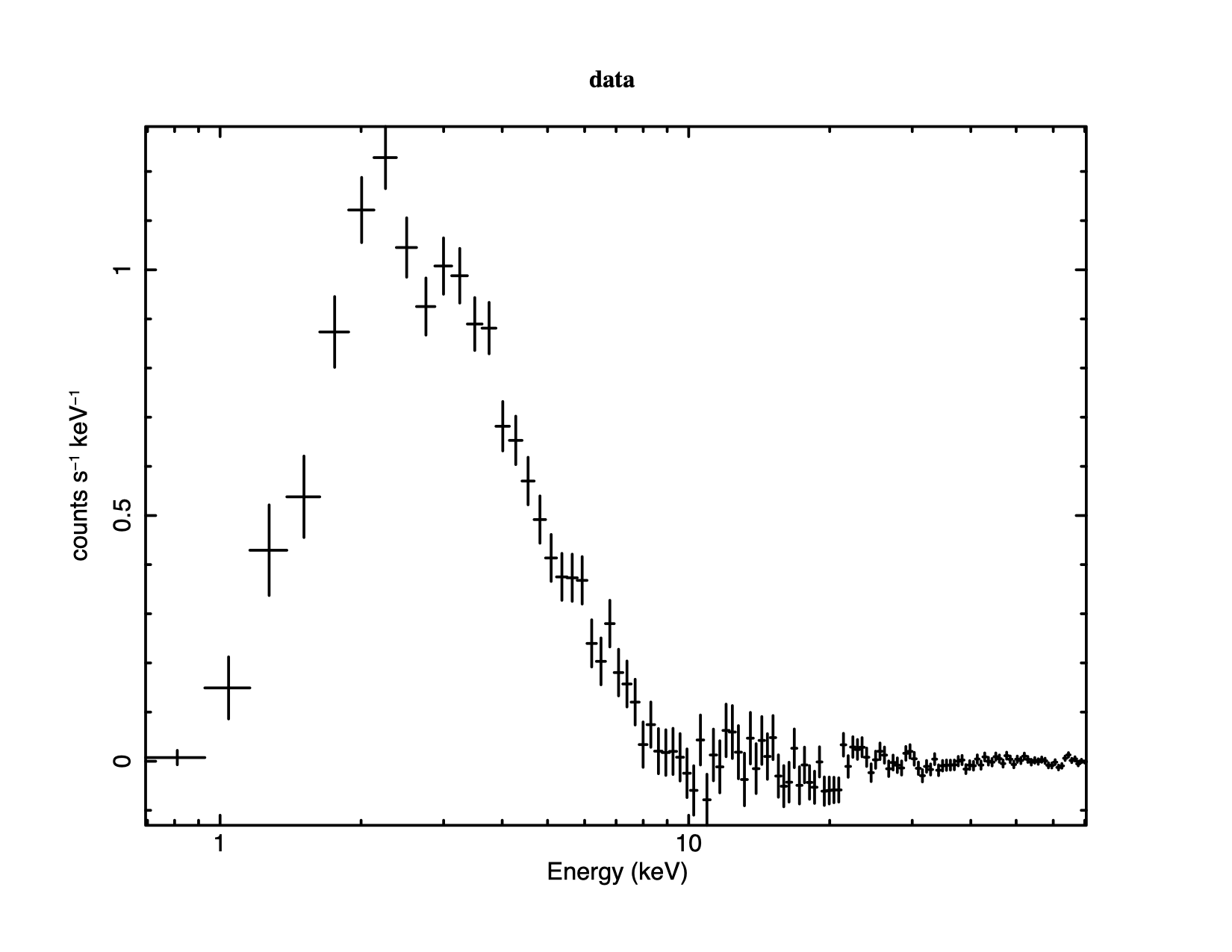
The most fundamental is the data plotted against instrument channel (data); next most fundamental, and more informative, is the data plotted against channel energy. To do this plot, use the XSPEC command setplot energy. Figure 4.1 shows the result of the commands:
XSPEC12> setplot energy
XSPEC12> plot data
Note the label on the y-axis has no cm We are now ready to fit the data with a model. Models in XSPEC are specified using the model command, followed by an algebraic expression of a combination of model components. There are two basic kinds of model components: additive and multiplicative. Additive components represent X-Ray sources of different kinds (e.g., a bremsstrahlung continuum) and, after being convolved with the instrument response, prescribe the number of counts per energy bin. Multiplicative components represent phenomena that modify the observed X-Radiation (e.g. reddening or an absorption edge). They apply an energy-dependent multiplicative factor to the source radiation before the result is convolved with the instrumental response.
More generally, XSPEC allows three types of modifying components: convolutions and mixing models in addition to the multiplicative type. Since there must be a source, there must be least one additive component in a model, but there is no restriction on the number of modifying components. To see what components are available, just type model :
XSPEC12>model
Additive Models:
agauss      c6vmekl     eqpair      nei         rnei        vraymond
agnsed      carbatm     eqtherm     nlapec      sedov       vrnei
agnslim     cemekl      equil       npshock     sirf        vsedov
apec        cevmkl      expdec      nsa         slimbh      vtapec
bapec       cflow       ezdiskbb    nsagrav     smaug       vvapec
bbody       compLS      gadem       nsatmos     snapec      vvgnei
bbodyrad    compPS      gaussian    nsmax       srcut       vvnei
bexrav      compST      gnei        nsmaxg      sresc       vvnpshock
bexriv      compTT      grad        nsx         ssa         vvpshock
bkn2pow     compbb      grbcomp     nteea       step        vvrnei
bknpower    compmag     grbjet      nthComp     tapec       vvsedov
bmc         comptb      grbm        optxagn     vapec       vvtapec
bremss      compth      hatm        optxagnf    vbremss     vvwdem
brnei       cph         jet         pegpwrlw    vcph        vwdem
btapec      cplinear    kerrbb      pexmon      vequil      wdem
bvapec      cutoffpl    kerrd       pexrav      vgadem      zagauss
bvrnei      disk        kerrdisk    pexriv      vgnei       zbbody
bvtapec     diskbb      kyrline     plcabs      vmcflow     zbknpower
bvvapec     diskir      laor        posm        vmeka       zbremss
bvvrnei     diskline    laor2       powerlaw    vmekal      zcutoffpl
bvvtapec    diskm       logpar      pshock      vnei        zgauss
bwcycl      disko       lorentz     qsosed      vnpshock    zkerrbb
c6mekl      diskpbb     meka        raymond     voigt       zlogpar
c6pmekl     diskpn      mekal       redge       vpshock     zpowerlw
c6pvmkl     eplogpar    mkcflow     refsch


Multiplicative Models:
SSS_ice     constant    ismdust     polpow      wndabs      zphabs
TBabs       cyclabs     log10con    pwab        xion        zredden
TBfeo       dust        logconst    redden      xscat       zsmdust
TBgas       edge        lyman       smedge      zTBabs      zvarabs
TBgrain     expabs      notch       spexpcut    zbabs       zvfeabs
TBpcf       expfac      olivineabs  spline      zdust       zvphabs
TBrel       gabs        pcfabs      swind1      zedge       zwabs
TBvarabs    heilin      phabs       uvred       zhighect    zwndabs
absori      highecut    plabs       varabs      zigm        zxipab
acisabs     hrefl       polconst    vphabs      zpcfabs     zxipcf
cabs        ismabs      pollin      wabs


Convolution Models:
cflux       ireflect    kyconv      reflect     thcomp      xilconv
clumin      kdblur      lsmooth     rfxconv     vashift     zashift
cpflux      kdblur2     partcov     rgsxsrc     vmshift     zmshift
gsmooth     kerrconv    rdblur      simpl


Mixing Models:
ascac       monomass    polrot      recorn      suzpsf      xmmpsf
clmass      nfwmass     projct


Pile-up Models:
pileup


Table models may be used with the commands atable/mtable/etable
atable{</path/to/tablemodel.mod>}
and are described at:
heasarc.gsfc.nasa.gov/docs/heasarc/ofwg/docs/general/ogip_92_009/ogip_92_009.html

Additional models are available at:
heasarc.gsfc.nasa.gov/docs/xanadu/xspec/newmodels.html
For information about a specific component, type help model followed by the name of the component:
XSPEC12>help model apec Given the quality of our data, as shown by the plot, we'll choose an absorbed power law, specified as follows :
XSPEC12> model phabs(powerlaw) Or, abbreviating unambiguously:
XSPEC12> mo pha(po)
The user is then prompted for the initial values of the
parameters. Entering
XSPEC12>mo pha(po)

Input parameter value, delta, min, bot, top, and max values for ...
              1      0.001(      0.01)          0          0     100000   1E+06
1:phabs:nH>/*

========================================================================
Model: phabs<1>*powerlaw<2> Source No.: 1  Active/On
Model  Model Component  Parameter  Unit    Value
 par  comp
  1     1    phabs      nH         10^22   1.00000       +/-  0.0
  2     2    powerlaw   PhoIndex           1.00000       +/-  0.0
  3     2    powerlaw   norm               1.00000       +/-  0.0
 ________________________________________________________________________


Fit statistic  : Chi-Squared              4.878354e+08     using 125 bins.

Test statistic : Chi-Squared              4.878354e+08     using 125 bins.
 Null hypothesis probability of 0.000000e+00 with 122 degrees of freedom
 Current data and model not fit yet.
The current statistic is
XSPEC12> renorm

Fit statistic  : Chi-Squared                  845.91     using 125 bins.

Test statistic : Chi-Squared                  845.91     using 125 bins.
 Null hypothesis probability of 1.09e-108 with 122 degrees of freedom
 Current data and model not fit yet.
We are not quite ready to fit the data (and obtain a better
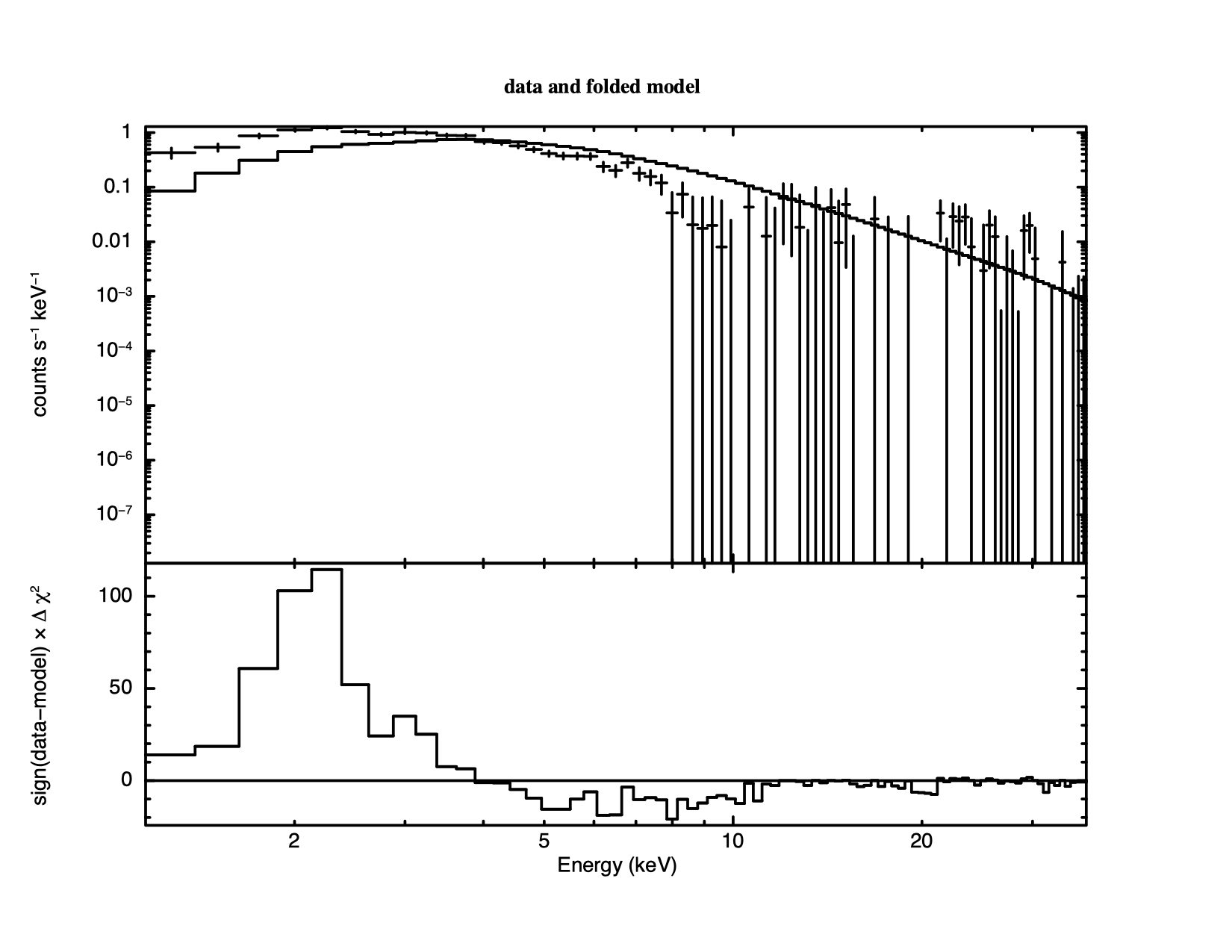
XSPEC12> ignore bad

ignore:    40 channels ignored from  source number 1
Fit statistic  : Chi-Squared                  793.46     using 85 bins.

Test statistic : Chi-Squared                  793.46     using 85 bins.
 Null hypothesis probability of 5.97e-117 with 82 degrees of freedom
 Current data and model not fit yet.
Then plot with:
XSPEC12> plot ldata chi We get a warning that the fit is not current because no fit has been performed yet.
Giving two options for the plot command generates a plot with
vertically stacked windows. Up to six options can be given to the plot
command at a time. Forty channels were rejected because they were
flagged as bad – but do we need to ignore any more? Figure
4.2 shows the result of plotting the data and the model
(in the upper window) and the contributions to
XSPEC12> ignore 15.0-**
     78 channels (48-125) ignored in spectrum #     1

Fit statistic  : Chi-Squared                  715.30     using 45 bins.

Test statistic : Chi-Squared                  715.30     using 45 bins.
 Null hypothesis probability of 2.42e-123 with 42 degrees of freedom
 Current data and model not fit yet.
If the ignore command is handed a real number it assumes energy in keV while if it is handed an integer it will assume channel number. The “**” just means the highest energy. Starting a range with “**” means the lowest energy. The inverse of ignore is notice, which has the same syntax.
We are now ready to fit the data. Fitting is initiated by the command
fit. As the fit proceeds, the screen displays the status of the fit
for each iteration until either the fit converges to the minimum
XSPEC12>fit
Parameters
Chi-Squared  |beta|/N    Lvl          1:nH    2:PhoIndex        3:norm
450.421      150.593      -3     0.0916817       1.61266    0.00388600
412.275      63000.6      -3      0.283518       2.30662    0.00911916
53.9571      27976.3      -4      0.529631       2.14207     0.0121535
43.8301      4648.87      -5      0.565375       2.23873     0.0130851
43.8179      125.675      -6      0.552335       2.23611     0.0130313
43.8179      0.622244     -7      0.551351       2.23578     0.0130239
========================================
Variances and Principal Axes
1        2        3
4.7830E-08| -0.0025  -0.0151   0.9999
2.3114E-03|  0.3929  -0.9195  -0.0129
9.0741E-02|  0.9196   0.3928   0.0082
----------------------------------------

====================================
Covariance Matrix
1           2           3
7.709e-02   3.194e-02   6.736e-04
3.194e-02   1.595e-02   3.201e-04
6.736e-04   3.201e-04   6.553e-06
------------------------------------

========================================================================
Model phabs<1>*powerlaw<2> Source No.: 1   Active/On
Model Model Component  Parameter  Unit     Value
par  comp
1    1   phabs      nH         10^22    0.551351     +/-  0.277654
2    2   powerlaw   PhoIndex            2.23578      +/-  0.126308
3    2   powerlaw   norm                1.30239E-02  +/-  2.55995E-03
________________________________________________________________________


Fit statistic  : Chi-Squared                   43.82     using 45 bins.

Test statistic : Chi-Squared                   43.82     using 45 bins.
 Null hypothesis probability of 3.94e-01 with 42 degrees of freedom
There is a fair amount of information here so we will unpack it a bit
at a time. One line is written out after each fit iteration. The
columns labeled Chi-Squared and Parameters are obvious. The other two
provide additional information on fit convergence. At each step in the
fit a numerical derivative of the statistic with respect to the
parameters is calculated. We call the vector of these derivatives
beta. At the best-fit the norm of beta should be zero so we write out
At the end of the fit XSPEC writes out the Variances and Principal Axes and Covariance Matrix sections. These are both based on the second derivatives of the statistic with respect to the parameters. Generally, the larger these second derivatives, the better determined the parameter (think of the case of a parabola in 1-D). The Covariance Matrix is the inverse of the matrix of second derivatives. The Variances and Principal Axes section is based on an eigenvector decomposition of the matrix of second derivatives and indicates which parameters are correlated. We can see in this case that the first eigenvector depends almost entirely on the powerlaw norm while the other two are combinations of the nH and powerlaw PhoIndex. This tells us that the norm is independent but the other two parameters are correlated. The next section shows the best-fit parameters and error estimates. The latter are just the square roots of the diagonal elements of the covariance matrix so implicitly assume that the parameter space is multidimensional Gaussian with all parameters independent. We already know in this case that the parameters are not independent so these error estimates should only be considered guidelines to help us determine the true errors later.
The final section shows the statistic values at the end of the
fit. XSPEC defines a fit statistic, used to determine the best-fit
parameters and errors, and test statistic, used to decide whether this
model and parameters provide a good fit to the data. By default, both
statistics are
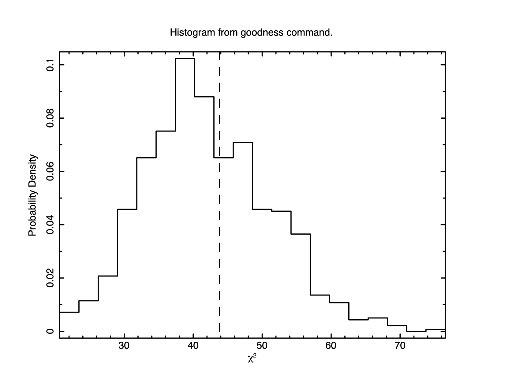
XSPEC12>goodness 1000
Parameter distribution is derived from fit covariance matrix.
61.20% of realizations are < best test statistic 43.82  (sim)  (fit)
XSPEC12>plot goodness
A little more than half of the simulations give a statistic value less
than that observed, consistent with this being a good fit. Figure
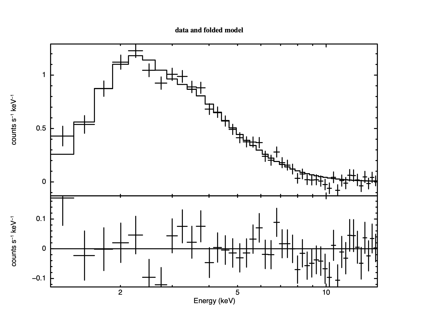
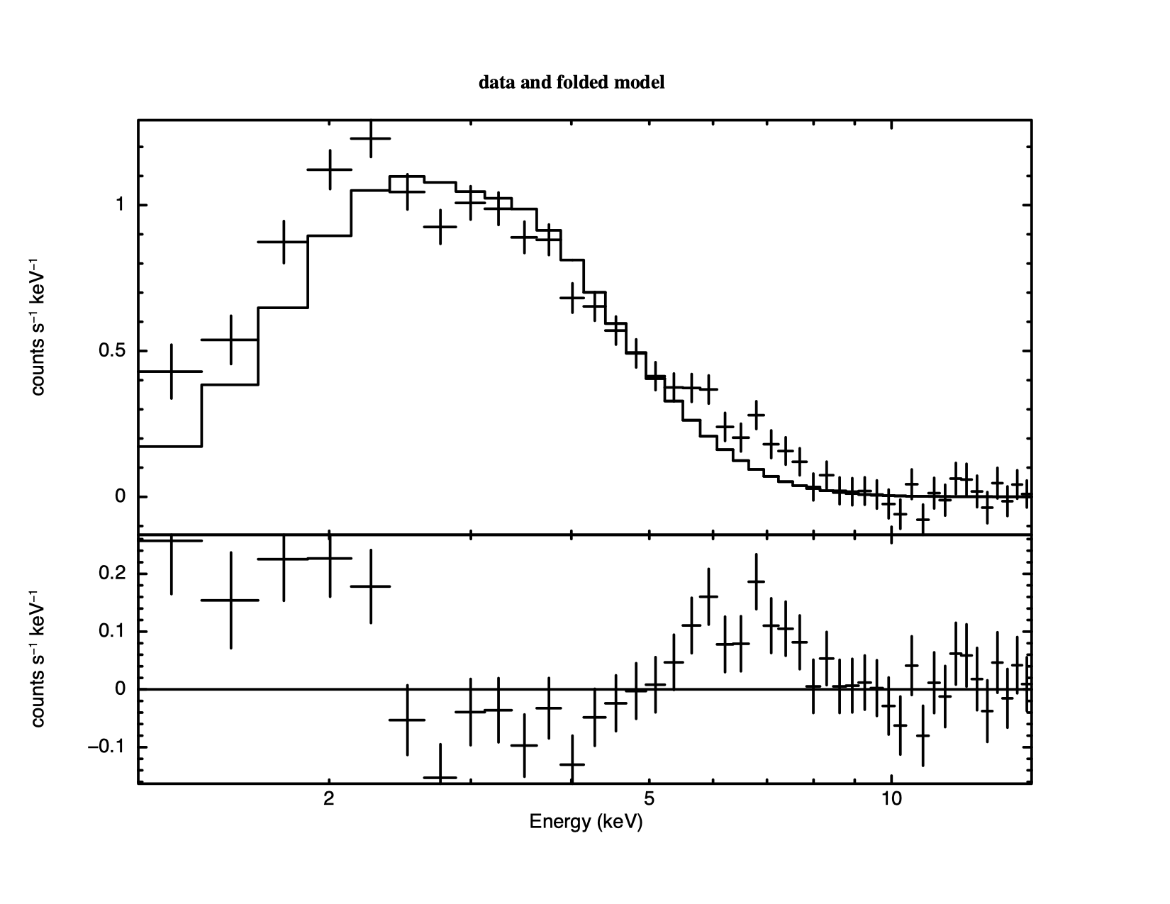
4.3 shows a histogram of the So the statistic implies the fit is good but it is still always a good idea to look at the data and residuals to check for any systematic differences that may not be caught by the test. To see the fit and the residuals, we produce figure 4.4 using the command
XSPEC12>plot data resid
Now that we think we have the correct model we need to determine how well the parameters are determined. The screen output at the end of the fit shows the best-fitting parameter values, as well as approximations to their errors. These errors should be regarded as indications of the uncertainties in the parameters and should not be quoted in publications. The true errors, i.e. the confidence ranges, are obtained using the error command. We want to run error on all three parameters which is an intrinsically parallel operation so we can use XSPEC's support for multiple cores and run the error estimations in parallel:
XSPEC12>parallel error 3
XSPEC12>error 1 2 3
 Parameter   Confidence Range (2.706)
     1     0.109522      1.03334    (-0.441776,0.482041)
     2      2.03727      2.44823    (-0.198497,0.212462)
     3   0.00953569    0.0181505    (-0.00348792,0.00512687)
Here, the numbers 1, 2, 3 refer to the parameter numbers in the Model
par column of the output at the end of the fit. For the first
parameter, the column of absorbing hydrogen atoms, the 90% confidence
range is
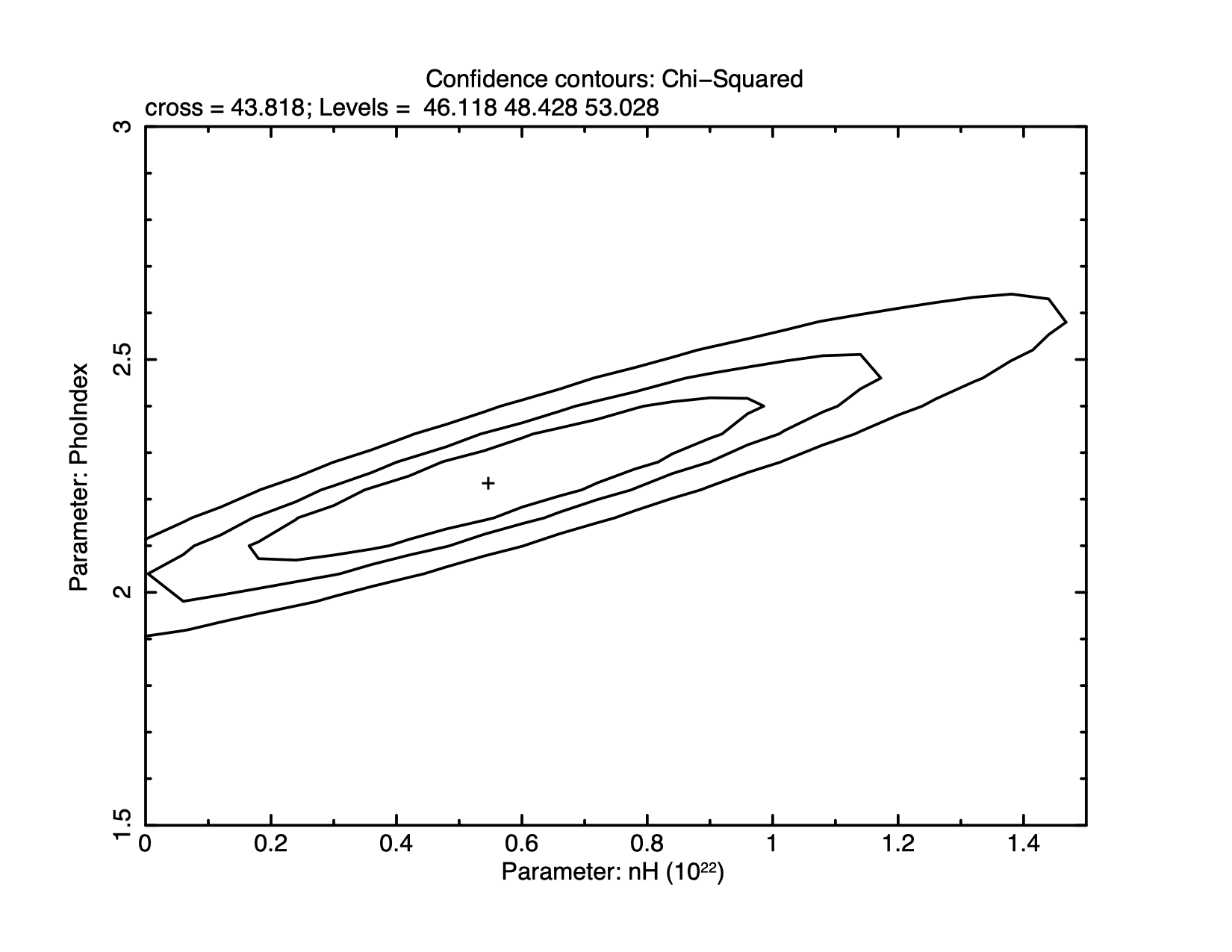
XSPEC12>steppar 1 0.0 1.5 25 2 1.5 3.0 25

     Chi-Squared    Delta               nH      PhoIndex
                 Chi-Squared             1             2

          162.65      118.83    0           0    0         1.5
          171.34      127.53    1        0.06    0         1.5
          180.35      136.53    2        0.12    0         1.5
          189.64      145.82    3        0.18    0         1.5
           199.2      155.38    4        0.24    0         1.5
                 . . . . . . .
          318.01       274.2    4        0.24   25           3
          336.24      292.42    3        0.18   25           3
          355.29      311.47    2        0.12   25           3
          375.18      331.37    1        0.06   25           3
          395.94      352.12    0           0   25           3
and make the contour plot shown in figure 4.5 using:
XSPEC12>plot contour
What else can we do with the fit? One thing is to derive the flux of the model. The data by themselves only give the instrument-dependent count rate. The model, on the other hand, is an estimate of the true spectrum emitted. In XSPEC, the model is defined in physical units independent of the instrument. The command flux integrates the current model over the range specified by the user:
XSPEC12> flux 2 10
  Model Flux  0.0035392 photons (2.2323e-11 ergs/cm^2/s) range (2.0000 - 10.000 keV)
Here we have chosen the standard X-ray range of 2–10 keV and find that
the energy flux is
XSPEC12>energies extend low 0.2 100

Models will use response energies extended to:
   Low:  0.2 in 100 log bins

Fit statistic  : Chi-Squared                   43.82     using 45 bins.

Test statistic : Chi-Squared                   43.82     using 45 bins.
 Null hypothesis probability of 3.94e-01 with 42 degrees of freedom
 Current data and model not fit yet.

XSPEC12>flux 0.2 2.
  Model Flux  0.0042889 photons (8.7877e-12 ergs/cm^2/s) range (0.20000 - 2.0000 keV)
The energy flux, at
XSPEC12>editmod pha*cflux(pow)

Input parameter value, delta, min, bot, top, and max values for ...
            0.5       -0.1(     0.005)          0          0      1e+06      1e+06
2:cflux:Emin>0.2
             10       -0.1(       0.1)          0          0      1e+06      1e+06
3:cflux:Emax>2.0
            -12       0.01(      0.12)       -100       -100        100        100
4:cflux:lg10Flux>-10.3

Fit statistic  : Chi-Squared                   51.71     using 45 bins.

Test statistic : Chi-Squared                   51.71     using 45 bins.
 Null hypothesis probability of 1.22e-01 with 41 degrees of freedom
 Current data and model not fit yet.

========================================================================
Model phabs<1>*cflux<2>*powerlaw<3> Source No.: 1   Active/On
Model Model Component  Parameter  Unit     Value
 par  comp
   1    1   phabs      nH         10^22    0.551483     +/-  0.277863
   2    2   cflux      Emin       keV      0.200000     frozen
   3    2   cflux      Emax       keV      2.00000      frozen
   4    2   cflux      lg10Flux   cgs      -10.3000     +/-  0.0
   5    3   powerlaw   PhoIndex            2.23579      +/-  0.126392
   6    3   powerlaw   norm                1.30242E-02  +/-  2.57317E-03

________________________________________________________________________
The Emin and Emax parameters are set to the energy range over which we want the flux to be calculated. We also have to fix the norm of the powerlaw because the normalization of the model will now be determined by the lg10Flux parameter. This is done using the freeze command:
XSPEC12>freeze 6 We now run fit to get the best-fit value of lg10Flux as -10.2792:
XSPEC12>fit
 Warning: renorm - no variable model to allow  renormalization
                                   Parameters
Chi-Squared  |beta|/N    Lvl          1:nH    4:lg10Flux    5:PhoIndex
43.821       153.715      -3      0.542840      -10.2824       2.23172
43.8179      2.65056      -4      0.550962      -10.2792       2.23570
========================================
 Variances and Principal Axes
                 1        4        5
 3.3544E-05|  0.0629  -0.8010   0.5954
 3.1521E-03|  0.5045  -0.4892  -0.7114
 1.0233E-01|  0.8611   0.3451   0.3733
----------------------------------------

====================================
  Covariance Matrix
        1           2           3
   7.669e-02   2.963e-02   3.177e-02
   2.963e-02   1.296e-02   1.427e-02
   3.177e-02   1.427e-02   1.587e-02
------------------------------------

========================================================================
Model phabs<1>*cflux<2>*powerlaw<3> Source No.: 1   Active/On
Model Model Component  Parameter  Unit     Value
 par  comp
   1    1   phabs      nH         10^22    0.550962     +/-  0.276921
   2    2   cflux      Emin       keV      0.200000     frozen
   3    2   cflux      Emax       keV      2.00000      frozen
   4    2   cflux      lg10Flux   cgs      -10.2792     +/-  0.113860
   5    3   powerlaw   PhoIndex            2.23570      +/-  0.125973
   6    3   powerlaw   norm                1.30242E-02  frozen
________________________________________________________________________


Fit statistic  : Chi-Squared                   43.82     using 45 bins.

Test statistic : Chi-Squared                   43.82     using 45 bins.
 Null hypothesis probability of 3.94e-01 with 42 degrees of freedom
Then find the error on that parameter:
XSPEC12>error 4
 Parameter   Confidence Range (2.706)
     4      -10.4578    -10.0801    (-0.178718,0.198982)
for a 90% confidence range on the 0.2–2 keV unabsorbed flux of
The fit, as we've remarked, is good, and the parameters are constrained. But unless the purpose of our investigation is merely to measure a photon index, it's a good idea to check whether alternative models can fit the data just as well. We also should derive upper limits to components such as iron emission lines and additional continua, which, although not evident in the data nor required for a good fit, are nevertheless important to constrain. First, let's try an absorbed black body:
XSPEC12>mo pha(bb)

Input parameter value, delta, min, bot, top, and max values for ...
              1      0.001(      0.01)          0          0     100000      1e+06
1:phabs:nH>/*

========================================================================
Model phabs<1>*bbody<2> Source No.: 1   Active/On
Model Model Component  Parameter  Unit     Value
 par  comp
   1    1   phabs      nH         10^22    1.00000      +/-  0.0
   2    2   bbody      kT         keV      3.00000      +/-  0.0
   3    2   bbody      norm                1.00000      +/-  0.0
________________________________________________________________________


Fit statistic : Chi-Squared =   3.377094e+09 using 45 PHA bins.

Test statistic : Chi-Squared =   3.377094e+09 using 45 PHA bins.
 Reduced chi-squared =   8.040700e+07 for     42 degrees of freedom
 Null hypothesis probability =   0.000000e+00
 Current data and model not fit yet.
XSPEC12>fit
                                   Parameters
Chi-Squared  |beta|/N    Lvl          1:nH          2:kT        3:norm
1532.94      63.1918       0      0.332069       3.01550   0.000673517
1521.42      111571        0      0.153909       2.96509   0.000613317
1490.16      170627        0     0.0624033       2.87563   0.000569789
1443.32      204857        0     0.0178739       2.76602   0.000534628
1388.24      227421        0    0.00734630       2.64698   0.000503822
1324.93      244501        0    0.00243756       2.52364   0.000475538
1254.69      259287        0   0.000178082       2.39808   0.000449095
1178.52      272841        0   5.59277e-05       2.27059   0.000423584
1085.63      287146        0   2.59575e-05       2.13543   0.000401354
985.199      290402        0   1.33741e-06       1.99739   0.000379210
Number of trials exceeded: continue fitting? Y
 ...
 ...
123.773      23.7694      -3   6.35802e-09      0.890290   0.000278598
Number of trials exceeded: continue fitting?
***Warning: Zero alpha-matrix diagonal element for parameter 1
 Parameter 1 is pegged at 6.35802e-09 due to zero or negative pivot element, likely
 caused by the fit being insensitive to the parameter.
123.773      0.374813     -3   6.35802e-09      0.890204   0.000278596
==============================
 Variances and Principal Axes
                 2        3
 2.2370E-11| -0.0000   1.0000
 2.8677E-04|  1.0000   0.0000
------------------------------

========================
  Covariance Matrix
        1           2
   2.868e-04   9.336e-09
   9.336e-09   2.267e-11
------------------------

========================================================================
Model phabs<1>*bbody<2> Source No.: 1   Active/On
Model Model Component  Parameter  Unit     Value
 par  comp
   1    1   phabs      nH         10^22    6.35802E-09  +/-  -1.00000
   2    2   bbody      kT         keV      0.890204     +/-  1.69342E-02
   3    2   bbody      norm                2.78596E-04  +/-  4.76175E-06
________________________________________________________________________


Fit statistic  : Chi-Squared                  123.77     using 45 bins.

Test statistic : Chi-Squared                  123.77     using 45 bins.
 Null hypothesis probability of 5.42e-10 with 42 degrees of freedom
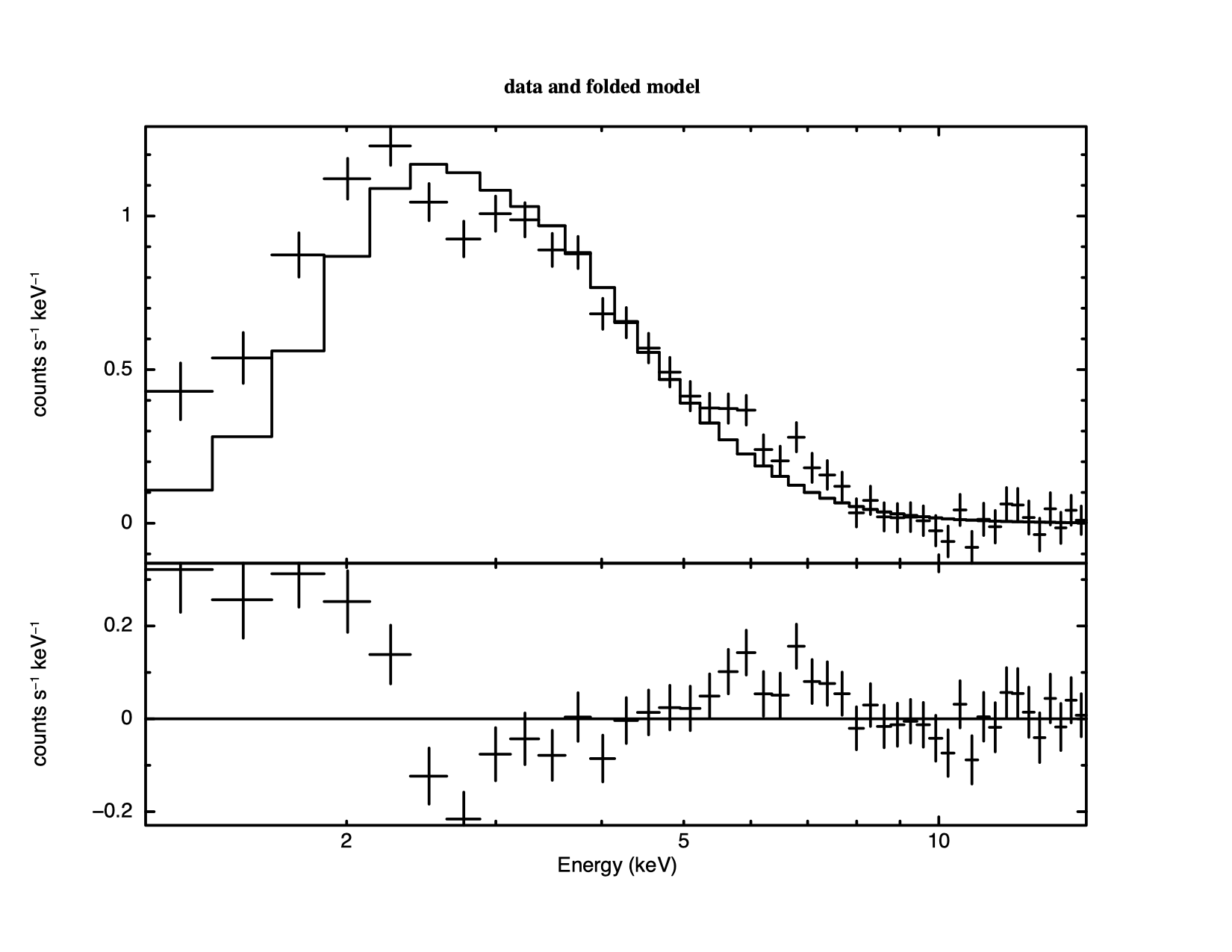
Note that after each set of 10 iterations you are asked whether you want to continue. Replying no at these prompts is a good idea if the fit is not converging quickly. Conversely, to avoid having to keep answering the question, i.e., to increase the number of iterations before the prompting question appears, begin the fit with, say fit 100. This command will put the fit through 100 iterations before pausing. To automatically answer yes to all such questions use the command query yes. Note that the fit has written out a warning about the first parameter and its estimated error is written as -1. This indicates that the fit is unable to constrain the parameter and it should be considered indeterminate. This usually indicates that the model is not appropriate. One thing to check in this case is that the model component has any contribution within the energy range being calculated. Plotting the data and residuals again we obtain Figure 4.6.
The black body fit is obviously not a good one. Not only is
Let's try thermal bremsstrahlung next:
XSPEC12>mo pha(br)
Input parameter value, delta, min, bot, top, and max values for ...
              1      0.001(      0.01)          0          0     100000      1e+06
1:phabs:nH>/*

========================================================================
Model phabs<1>*bremss<2> Source No.: 1   Active/On
Model Model Component  Parameter  Unit     Value
 par  comp
   1    1   phabs      nH         10^22    1.00000      +/-  0.0
   2    2   bremss     kT         keV      7.00000      +/-  0.0
   3    2   bremss     norm                1.00000      +/-  0.0
________________________________________________________________________


Fit statistic  : Chi-Squared              4.561670e+07     using 45 bins.

Test statistic : Chi-Squared              4.561670e+07     using 45 bins.
 Null hypothesis probability of 0.000000e+00 with 42 degrees of freedom
 Current data and model not fit yet.
XSPEC12>fit
                                   Parameters
Chi-Squared  |beta|/N    Lvl          1:nH          2:kT        3:norm
102.905      23.3691      -3      0.274774       6.15759    0.00726465
46.547       16309.7      -4     0.0366323       5.60534    0.00785786
...
...
42.3441      3135.61      -8   1.65741e-06       5.64294    0.00792237
========================================
 Variances and Principal Axes
                 1        2        3
 1.8456E-08| -0.0015   0.0006   1.0000
 1.3122E-02|  0.9776   0.2103   0.0013
 6.6860E-01| -0.2103   0.9776  -0.0009
----------------------------------------

====================================
  Covariance Matrix
        1           2           3
   4.211e-02  -1.348e-01   1.388e-04
  -1.348e-01   6.396e-01  -5.632e-04
   1.388e-04  -5.632e-04   5.441e-07
------------------------------------

========================================================================
Model phabs<1>*bremss<2> Source No.: 1   Active/On
Model Model Component  Parameter  Unit     Value
 par  comp
   1    1   phabs      nH         10^22    1.65741E-06  +/-  0.205196
   2    2   bremss     kT         keV      5.64294      +/-  0.799757
   3    2   bremss     norm                7.92237E-03  +/-  7.37654E-04
________________________________________________________________________


Fit statistic  : Chi-Squared                   42.34     using 45 bins.

Test statistic : Chi-Squared                   42.34     using 45 bins.
 Null hypothesis probability of 4.56e-01 with 42 degrees of freedom
Bremsstrahlung is a better fit than the black body – and is as good as
the power law – although it shares the low N First, we reset our fit to the powerlaw (output omitted):
XSPEC12>mo pha(po)
From the EXOSAT database on HEASARC, we know that the target in
question, 1E1048.1–5937, has a Galactic latitude of 24 arcmin, i.e., almost on
the plane of the Galaxy. In fact, the database also provides the value
of the Galactic N
XSPEC12> freeze 1 The inverse of freeze is thaw:
XSPEC12> thaw 1
Alternatively, parameters can be frozen using the newpar
command, which allows all the quantities associated with a parameter
to be changed. We can flip between frozen and thawed states by
entering 0 after the new parameter value. In our case, we want N
XSPEC12>newpar 1
Current value, delta, min, bot, top, and max values
       0.551351      0.001(0.00551351)          0          0     100000      1e+06
1:phabs[1]:nH:1>4,0

Fit statistic  : Chi-Squared                  800.74     using 45 bins.

Test statistic : Chi-Squared                  800.74     using 45 bins.
 Null hypothesis probability of 2.82e-140 with 43 degrees of freedom
 Current data and model not fit yet.
The same result can be obtained by putting everything onto the command line, i.e., newpar 1 4, 0, or by issuing the two commands, newpar 1 4 followed by freeze 1. Now, if we fit and plot again, we get the following model (Fig. 4.7).
XSPEC12>fit
...
 ========================================================================
Model phabs<1>*powerlaw<2> Source No.: 1   Active/On
Model Model Component  Parameter  Unit     Value
 par  comp
   1    1   phabs      nH         10^22    4.00000      frozen
   2    2   powerlaw   PhoIndex            3.55530      +/-  6.72007E-02
   3    2   powerlaw   norm                0.109349     +/-  8.78816E-03
________________________________________________________________________


Fit statistic  : Chi-Squared                  131.82     using 45 bins.
The fit is not good. In Figure 4.7 we can see why: there appears to be a surplus of softer photons, perhaps indicating a second continuum component. To investigate this possibility we can add a component to our model. The editmod command lets us do this without having to respecify the model from scratch. Here, we'll add a black body component.
XSPEC12>editmod pha(po+bb)

Input parameter value, delta, min, bot, top, and max values for ...
              3       0.01(      0.03)     0.0001       0.01        100        200
4:bbody:kT>2,0
              1       0.01(      0.01)          0          0      1e+20      1e+24
5:bbody:norm>1e-5

Fit statistic  : Chi-Squared                  128.71     using 45 bins.

Test statistic : Chi-Squared                  128.71     using 45 bins.
 Null hypothesis probability of 9.87e-11 with 42 degrees of freedom
 Current data and model not fit yet.

========================================================================
Model phabs<1>(powerlaw<2> + bbody<3>)  Source No.: 1   Active/On
Model Model Component  Parameter  Unit      Value
 par  comp
   1    1   phabs      nH         10^22     4.00000      frozen
   2    2   powerlaw   PhoIndex             3.55530      +/-  6.72007E-02
   3    2   powerlaw   norm                 0.109349     +/-  8.78816E-03
   4    3   bbody      kT          keV      2.00000      frozen
   5    3   bbody      norm                 1.00000E-05  +/-  0.0

________________________________________________________________________
Notice that in specifying the initial values of the black body, we have frozen kT at 2 keV (the canonical temperature for nuclear burning on the surface of a neutron star in a low-mass X-ray binary) and started the normalization small. Without these measures, the fit might “lose its way”. Now, if we fit, we get (not showing all the iterations this time):
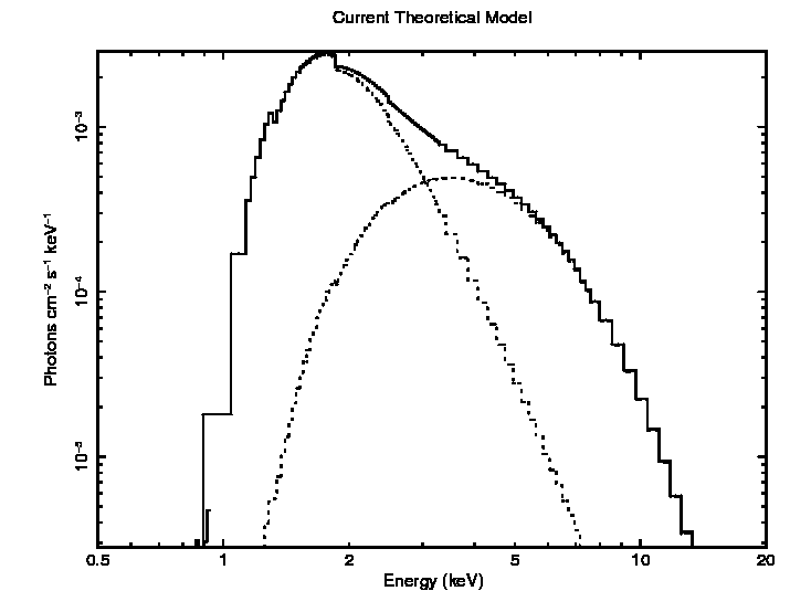
========================================================================
Model phabs<1>(powerlaw<2> + bbody<3>) Source No.: 1   Active/On
Model Model Component  Parameter  Unit     Value
 par  comp
   1    1   phabs      nH         10^22    4.00000      frozen
   2    2   powerlaw   PhoIndex            4.82939      +/-  0.159361
   3    2   powerlaw   norm                0.333962     +/-  4.81488E-02
   4    3   bbody      kT         keV      2.00000      frozen
   5    3   bbody      norm                2.27796E-04  +/-  2.06724E-05
________________________________________________________________________


Fit statistic : Chi-Squared                    68.45     using 45 PHA bins.
The fit is better than the one with just a power law and the fixed Galactic column, but it is still not good. Thawing the black body temperature and fitting does of course improve the fit but the powerl law index becomes even steeper. Looking at this odd model with the command
XSPEC12> plot model We see, in Figure 4.8, that the black body and the power law have changed places, in that the power law provides the soft photons required by the high absorption, while the black body provides the harder photons. We could continue to search for a plausible, well-fitting model, but the data, with their limited signal-to-noise and energy resolution, probably don't warrant it (the original investigators published only the power law fit).
There is, however, one final, useful thing to do with the data: derive
an upper limit to the presence of a fluorescent iron emission
line. First we delete the black body component using delcomp then
thaw N
========================================================================
Model phabs<1>(powerlaw<2> + gaussian<3>) Source No.: 1   Active/On
Model Model Component  Parameter  Unit     Value
 par  comp
   1    1   phabs      nH         10^22    0.772654     +/-  0.328763
   2    2   powerlaw   PhoIndex            2.38047      +/-  0.166698
   3    2   powerlaw   norm                1.58948E-02  +/-  3.94215E-03
   4    3   gaussian   LineE      keV      6.40000      frozen
   5    3   gaussian   Sigma      keV      0.100000     frozen
   6    3   gaussian   norm                7.46264E-05  +/-  4.74341E-05
________________________________________________________________________
The energy and width have to be frozen because, in the absence of an obvious line in the data, the fit would be completely unable to converge on meaningful values. Besides, our aim is to see how bright a line at 6.4 keV can be and still not ruin the fit. To do this, we fit first and then use the error command to derive the maximum allowable iron line normalization. We then set the normalization at this maximum value with newpar and, finally, derive the equivalent width using the eqwidth command. That is:
XSPEC12>err 6
 Parameter   Confidence Range (2.706)
***Warning: Parameter pegged at hard limit: 0
     6            0  0.000151075    (-7.46482e-05,7.64265e-05)
XSPEC12>new 6 0.000151075

Fit statistic  : Chi-Squared                   46.06     using 45 bins.

Test statistic : Chi-Squared                   46.06     using 45 bins.
 Null hypothesis probability of 2.71e-01 with 41 degrees of freedom
 Current data and model not fit yet.
XSPEC12>eqwidth 3

Data group number: 1
Additive group equiv width for Component 3:  0.782901 keV
Things to note:
Next: Simultaneous Fitting Up: Walks through XSPEC Previous: Brief Discussion of XSPEC HEASARC Home | Observatories | Archive | Calibration | Software | Tools | Students/Teachers/Public Last modified: Wednesday, 12-Mar-2025 17:05:25 EDT |