

CREATION OF EPIC BACKGROUND SUBTRACTED, EXPOSURE CORRECTED IMAGES
|
Introduction This thread describes how to create EPIC background subtracted, exposure corrected images combining data from the three instruments. A full guide to the use of the ESAS software can be found here.This thread uses data from the observation of Abell 1795, ObsID 0097820101, which is also used as the Imaging example where a script and output files are provided. Expected Outcome The final outcome of this thread are adaptively smoothed images in two spectral bands. In the process of creating the images full field of view and outer annulus spectral products (source and model background spectra, RMFs, and ARFs) are produced as well as count, exposure, and background count images.SAS Tasks to be Used
Prerequisites Useful Links
|
Procedure
This thread contains a step-by-step recipe to create EPIC background subtracted, exposure corrected images combining data from all three instruments.- Set up your SAS environment (following the SAS Startup Thread)
- Create cleaned (filtered for soft proton excesses) MOS and pn (including
OOT processing) event files for your observation:
epchain
epchain withoutoftime=true
emchain
pn-filter
mos-filter
Note that mos-filter indicates which CCDs are operating in an anomalous mode (the one marked by **** in the example below). These CCDs should be excluded in downstream processing.
1S003
Limit>1.5 CCD=2 Hardness=5.100 Uncertainty=0.882
Limit>1.5 CCD=3 Hardness=5.607 Uncertainty=1.150
Limit>2.5 CCD=4 Hardness=3.110 Uncertainty=0.418
Limit>2.5 CCD=5 Hardness=1.526 Uncertainty=0.149 ****
Limit>1.5 CCD=6 Hardness=4.000 Uncertainty=0.716
Limit>1.5 CCD=7 Hardness=5.629 Uncertainty=1.032
2S004
Limit>2.5 CCD=2 Hardness=2.639 Uncertainty=0.365
Limit>1.5 CCD=3 Hardness=4.419 Uncertainty=0.746
Limit>1.5 CCD=4 Hardness=6.875 Uncertainty=1.301
Limit>2.5 CCD=5 Hardness=3.982 Uncertainty=0.590
Limit>1.5 CCD=6 Hardness=4.432 Uncertainty=0.807
Limit>1.5 CCD=7 Hardness=4.600 Uncertainty=0.757
The diagnostic plots created by the filtering tasks should also be examined as they provide an indication of the quality of the data. These have names like mos1S003-hist.qdp, mos2S004-hist.qdp, and pnS005-hist.qdp and cam be plotted using the command, for example, qdp mos1S003-hist.qdp. Figure 1 shows the light-curve screening for the MOS1 instrument.
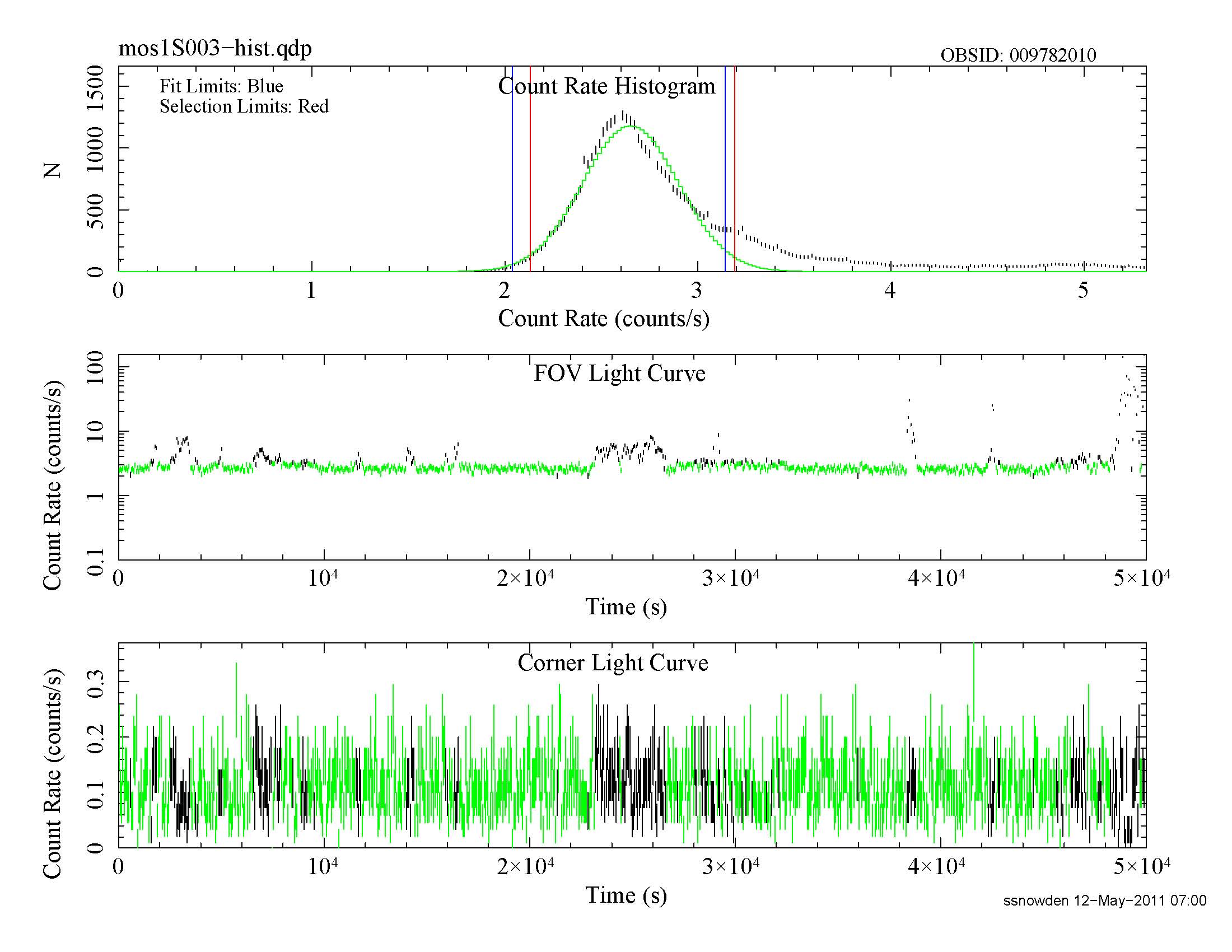
Figure 1: MOS1 light curve for the Abell 1795 observation. Notice the residual variation of the nominally good data which indicates the possible existence of residual soft proton contamination.
- Run source detection and make point-source masks. Note that in
this and many tasks below the exposure ID must be explicitly noted.
This is done by the prefixm, prefixp, and prefix
parameters.
cheese prefixm='1S003 2S004' prefixp=S005 scale=0.5 rate=1.0 dist=40.0 \
clobber=0 elow=400 ehigh=10000
- Examine the MOS soft band images to confirm that the indicated CCDs are
operating in an anomalous state, or that any other CCDs are doing so, and
verify that the point-source (cheese) masks look reasonable.
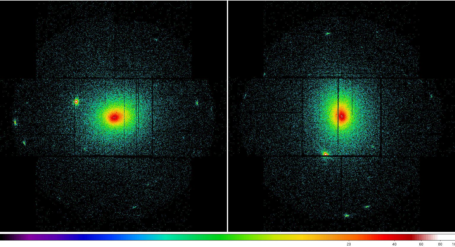
Figure 2: MOS1 (left) and MOS2 (right) images in the soft (0.2-1.0 keV) band. Note the excess counts in the upper left CCD in the MOS1 image most noticeable in the unexposed (to the sky) upper left corner. Displayed by the command: ds9 *soft* &.
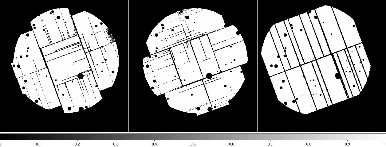
Figure 3: MOS1 (left), MOS2 (middle), and pn (right) cheese masks. Displayed by the command: ds9 *cheese* &
- Use
mos-spectra and
pn-spectra to create the
required intermediate spectra (for the entire region of interest
as well as spectra from the individual CCDs), RMF and ARF files, and
detector images for the two bands and three detectors. MOS CCDs
affected by anomalous states should
be deselected (this is done by the ccd# parameters).
MOS1 CCD6 should be deselected if the observation
took place after the meteorite damage. Currently the tasks require
the path to the additional CalDB files required for XMM-ESAS (in
this case, /PATH/esascaldb). The region selection
expression (region parameter) is in an input file and
should be in detector coordinates. If the input file does not exist,
reg.txt in this case, the default is to process the entire
FOV. The input energies are in eV.
mos-spectra prefix=1S003 caldb=/PATH/esascaldb region=reg.txt mask=1 \
elow=400 ehigh=1250 ccd1=1 ccd2=1 ccd3=1 ccd4=1 ccd5=0 ccd6=1 ccd7=1
mos-spectra prefix=1S003 caldb=/PATH/esascaldb region=reg.txt mask=1 \
elow=2000 ehigh=7200 ccd1=1 ccd2=1 ccd3=1 ccd4=1 ccd5=0 ccd6=1 ccd7=1
mos-spectra prefix=2S004 caldb=/PATH/esascaldb region=reg.txt mask=1 \
elow=400 ehigh=1250 ccd1=1 ccd2=1 ccd3=1 ccd4=1 ccd5=1 ccd6=1 ccd7=1
mos-spectra prefix=2S004 caldb=/PATH/esascaldb region=reg.txt mask=1 \
elow=2000 ehigh=7200 ccd1=1 ccd2=1 ccd3=1 ccd4=1 ccd5=1 ccd6=1 ccd7=1
pn-spectra prefix=S005 caldb=/software/XMM/CCF/esas region=pn-reg.txt \
mask=1 elow=400 ehigh=1250 pattern=4 quad1=1 quad2=1 quad3=1 quad4=1
pn-spectra prefix=S005 caldb=/software/XMM/CCF/esas region=pn-reg.txt \
mask=1 elow=2000 ehigh=7200 pattern=4 quad1=1 quad2=1 quad3=1 quad4=1
- Use
mos_back and
pn_back to create the quiescent
particle background (QPB) spectra and images (in detector coordinates).
mos_back and
pn_back create QDP plot files
which shows the source and model background spectra for the observation. Any
discrepancies at higher energies probably indicate residual soft proton
contamination, unless there are really hard and bright sources in the field.
In the case of this observation the discrepancy at high energies is consistent
with soft protons as a residual contamination was already expected from the light
curve histogram. The QDP files have names like mos1S005-spec.qdp. The
same CCD selection must be used here as were used in
mos-spectra and
pn-spectra.
mos_back prefix=1S003 caldb=/PATH/esascaldb diag=0 elow=400 ehigh=1250 \
ccd1=1 ccd2=1 ccd3=1 ccd4=1 ccd5=0 ccd6=1 ccd7=1
mos_back prefix=1S003 caldb=/PATH/esascaldb diag=0 elow=2000 ehigh=7200 \
ccd1=1 ccd2=1 ccd3=1 ccd4=1 ccd5=0 ccd6=1 ccd7=1
mos_back prefix=2S004 caldb=/PATH/esascaldb diag=0 elow=400 ehigh=1250 \
ccd1=1 ccd2=1 ccd3=1 ccd4=1 ccd5=1 ccd6=1 ccd7=1
mos_back prefix=2S004 caldb=/PATH/esascaldb diag=0 elow=2000 ehigh=7200 \
ccd1=1 ccd2=1 ccd3=1 ccd4=1 ccd5=1 ccd6=1 ccd7=1
pn_back prefix=S005 caldb=/PATH/esascaldb diag=0 elow=400 ehigh=1250 \
pattern=4 quad1=1 quad2=1 quad3=1 quad4=1
pn_back prefix=S005 caldb=/PATH/esascaldb diag=0 elow=2000 ehigh=7200 \
pattern=4 quad1=1 quad2=1 quad3=1 quad4=1
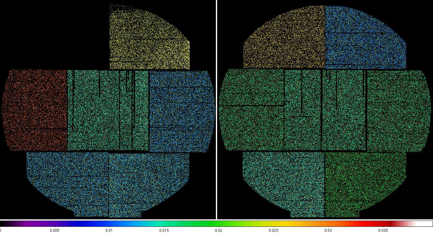
Figure 4: MOS1 (left) and MOS2 (right) model particle images in the soft (0.4-1.25 keV) band. The different colors for the different CCDs are an indication of the variations in their exposures (caused by CCDs operating in anomalous modes, CCD1 operating in non-full field imaging mode, and the loss of CCD6 of MOS1 to the micrometeorite strike. Displayed by the command: ds9 mos1S003-back-im-det-400-1250.fits mos2S004-back-im-det-400-1250.fits &.
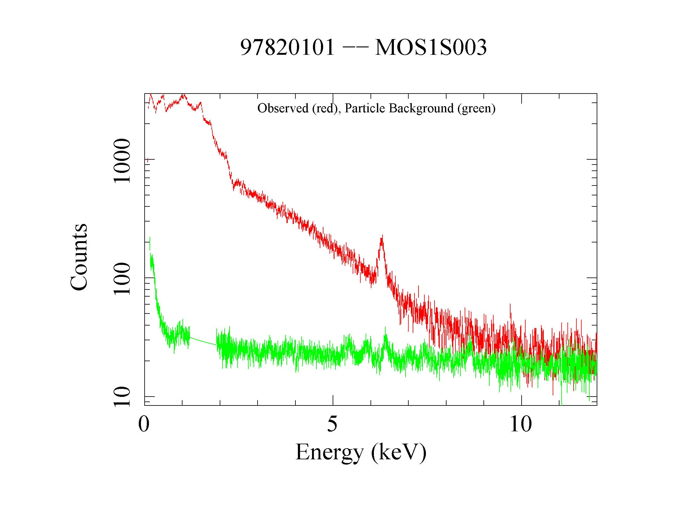
Figure 5: MOS1 source (red) and QPB (green) spectra. Displayed by the command: qdp mos1S003-spec.qdp.
- Use rot-im-det-sky
to transform the QPB images in detector coordinates into sky coordinates.
rot-im-det-sky prefix=1S003 mask=0 elow=400 ehigh=1250 mode=1
rot-im-det-sky prefix=1S003 mask=0 elow=2000 ehigh=7200 mode=1
rot-im-det-sky prefix=2S004 mask=0 elow=400 ehigh=1250 mode=1
rot-im-det-sky prefix=2S004 mask=0 elow=2000 ehigh=7200 mode=1
rot-im-det-sky prefix=S005 mask=0 elow=400 ehigh=1250 mode=1
rot-im-det-sky prefix=S005 mask=0 elow=2000 ehigh=7200 mode=1
- For convenience, rename a few files so that they are not overwritten.
mv mos1S003-obj.pi mos1S003-obj-full.pi
mv mos1S003.rmf mos1S003-full.rmf
mv mos1S003.arf mos1S003-full.arf
mv mos1S003-back.pi mos1S003-back-full.pi
mv mos1S003-obj-im-sp-det.fits mos1S003-sp-full.fits
mv mos2S004-obj.pi mos2S004-obj-full.pi
mv mos2S004.rmf mos2S004-full.rmf
mv mos2S004.arf mos2S004-full.arf
mv mos2S004-back.pi mos2S004-back-full.pi
mv mos2S004-obj-im-sp-det.fits mos2S004-sp-full.fits
mv pnS005-obj-os.pi pnS005-obj-os-full.pi
mv pnS005-obj.pi pnS005-obj-full.pi
mv pnS005-obj-oot.pi pnS005-obj-oot-full.pi
mv pnS005.rmf pnS005-full.rmf
mv pnS005.arf pnS005-full.arf
mv pnS005-back.pi pnS005-back-full.pi
mv pnS005-obj-im-sp-det.fits pnS005-sp-full.fits
- Group the spectral data in preparation for spectral fitting.
specgroup spectrumset=mos1S003-obj-full.pi mincounts=100 rmfset=mos1S003-full.rmf \
arfset=mos1S003-full.arf backgndset=mos1S003-back-full.pi groupedset=mos1S003-obj-full-grp.pi
specgroup spectrumset=mos2S004-obj-full.pi mincounts=100 rmfset=mos2S004-full.rmf \
arfset=mos2S004-full.arf backgndset=mos2S004-back-full.pi groupedset=mos2S004-obj-full-grp.pi
specgroup spectrumset=pnS005-obj-os-full.pi mincounts=100 rmfset=pnS005-full.rmf \
arfset=pnS005-full.arf backgndset=pnS005-back-full.pi groupedset=pnS005-obj-os-full-grp.pi
- Fit the spectral data to determine the soft proton contamination parameters.
This is aided by getting the ROSAT All-Sky Survey (RASS) spectrum of the region
from the HEASARC
X-ray background tool
along with the appropriate spectral response matrix
(rass.pi and
pspcc.rsp in this
Xspec XCM file).
The region selected for the RASS spectrum should be typical of the nominal
background in the direction of your source. For example, the spectrum in an
annulus surrounding a cluster of galaxies. The fitted model is fairly complex
with components representing the cosmic diffuse X-ray background (an unabsorbed
thermal component about 0.1 keV, and absorbed thermal component about 0.25 keV,
and the extragalactic power law with a spectral index of 1.46), a component
representing your source, Gaussian lines at 1.496 keV and 1.75 keV representing
the Al Kalpha and Si Kalpha lines in the MOS, lines at 1.496 keV and near 8 keV
representing the Al Kalpha and Cu lines in the pn, possible solar wind charge
exchange (SWCX) lines at 0.56 and 0.65 keV, and a power law representing the
residual soft proton contamination (MOS and pn only, fitted with a diagonal matrix
supplied in the XMM-ESAS CalDB release,
mos1-diag.rsp.gz,
mos2-diag.rsp.gz, and
pn-diag.rsp.gz).
The cosmic background parameters should be
linked for all spectra, your source spectrum parameters should be linked for
all spectra but the normalization should be fixed at 0 for the RASS data. The
SWCX parameters should be linked for all spectra but the normalization should
be fixed at 0 for the RASS data. The parameters for the soft proton background
should be independent except that the power law index for the two MOS detectors
can be linked. The non-detector components of the fit should be scaled by the
solid angle in square arc minutes (the RASS spectrum is already in these units).
proton_scale
finds the solid angle for the region to include in the spectral fitting.
proton_scale caldb=/PATH/esascaldb mode=1 detector=1 maskfile=mos1S003-sp-full.fits \
specfile=mos1S003-obj-full.pi
proton_scale caldb=/PATH/esascaldb mode=1 detector=2 maskfile=mos2S004-sp-full.fits \
specfile=mos2S004-obj-full.pi
proton_scale caldb=/PATH/esascaldb mode=1 detector=2 maskfile=pnS005-sp-full.fits \
specfile=pnS005-obj-full.pi
The result of the fitting process is shown if Figure 6.
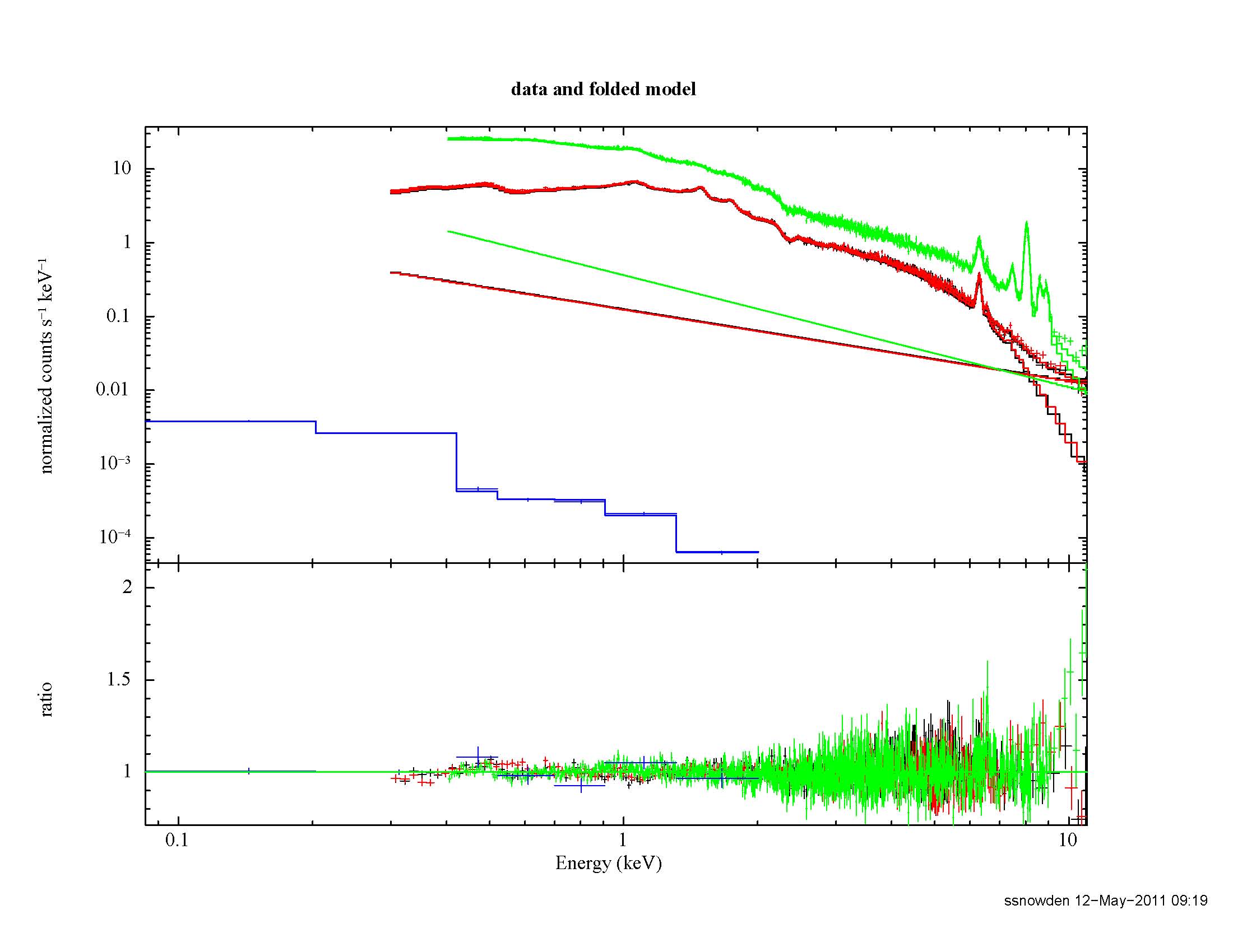
Figure 6: Best fit of the Abell 1795 data from the full FOV. The green data and model curves are from the pn, the black and red data and model curves are from the MOS1 and MOS2, respectively, and the blue model and curve are from the RASS. The straight line model curves for the MOS and pn are the soft proton contribution.
- proton uses the fitted soft proton parameters to create images of
the soft proton contamination in detector coordinates.
proton prefix=1S003 caldb=/PATH/esascaldb ccd1=1 ccd2=1 ccd3=1 ccd4=1 ccd5=1 \
ccd6=1 ccd7=1 elow=400 ehigh=1250 spectrumcontrol=1 pindex=0.963569 pnorm=0.126898
proton prefix=1S003 caldb=/PATH/esascaldb ccd1=1 ccd2=1 ccd3=1 ccd4=1 ccd5=1 \
ccd6=1 ccd7=1 elow=2000 ehigh=7200 spectrumcontrol=1 pindex=0.963569 pnorm=0.126898
proton prefix=2S004 caldb=/PATH/esascaldb ccd1=1 ccd2=1 ccd3=1 ccd4=1 ccd5=1 \
ccd6=1 ccd7=1 elow=400 ehigh=1250 spectrumcontrol=1 pindex=0.963569 pnorm=0.126718
proton prefix=2S004 caldb=/PATH/esascaldb ccd1=1 ccd2=1 ccd3=1 ccd4=1 ccd5=1 \
ccd6=1 ccd7=1 elow=2000 ehigh=7200 spectrumcontrol=1 pindex=0.963569 pnorm=0.126718
proton prefix=S005 caldb=/PATH/esascaldb ccd1=1 ccd2=1 ccd3=1 ccd4=1 \
elow=400 ehigh=1250 spectrumcontrol=1 pindex=1.51711 pnorm=0.339519
proton prefix=S005 caldb=/PATH/esascaldb ccd1=1 ccd2=1 ccd3=1 ccd4=1 \
elow=2000 ehigh=7200 spectrumcontrol=1 pindex=1.51711 pnorm=0.339519
- rot-im-det-sky
uses information in a previously created count image in sky
coordinates to rotate the detector coordinate soft proton background images into sky coordinates.
rot-im-det-sky prefix=1S003 mask=0 elow=400 ehigh=1250 mode=2
rot-im-det-sky prefix=1S003 mask=0 elow=2000 ehigh=7200 mode=2
rot-im-det-sky prefix=2S004 mask=0 elow=400 ehigh=1250 mode=2
rot-im-det-sky prefix=2S004 mask=0 elow=2000 ehigh=7200 mode=2
rot-im-det-sky prefix=S005 mask=0 elow=400 ehigh=1250 mode=2
rot-im-det-sky prefix=S005 mask=0 elow=2000 ehigh=7200 mode=2
At this point all of the components for all three instruments are ready to create and image. Figure 7 displays the components for MOS1.
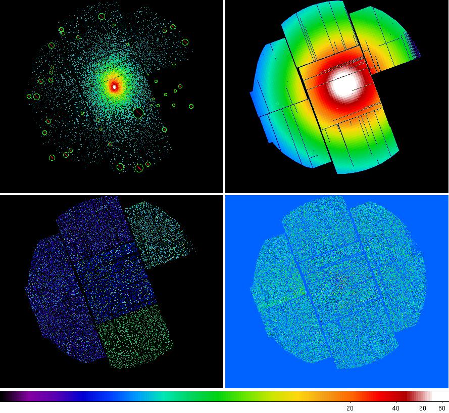
Figure 7: MOS1 image components with the count image which also shows the excluded point source regions (upper left), exposure image (upper right), QPB image (lower left), and soft proton image lower right.
- comb
combines the MOS1, MOS2, and pn images, as well as images from multiple
exposures. Since the spectra and images were created with point sources
removed comb must be run using the cheese masking.
comb caldb=/software/XMM/CCF/esas withpartcontrol=1 withsoftcontrol=1 withswcxcontrol=0 \
nbands=1 elowlist=400 ehighlist=1250 mask=1 ndata=3 prefixlist="1S003 2S004 S005"
comb caldb=/software/XMM/CCF/esas withpartcontrol=1 withsoftcontrol=1 withswcxcontrol=0 \
nbands=1 elowlist=2000 ehighlist=7200 mask=1 ndata=3 prefixlist="1S003 2S004 S005"
Figure 8 shows the merged component images.
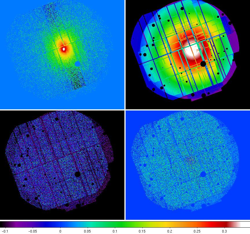
Figure 7: Merged image components with the count image (upper left), exposure image (upper right), QPB image (lower left), and soft proton image lower right. The negative counts in the count image are an artifact of the pn OOT correction.
- adapt_900 adaptively smooths the images.
adapt_900 smoothingcounts=50 thresholdmasking=0.02 detector=0 binning=2 elow=400 ehigh=1250 \
withpartcontrol=yes withsoftcontrol=yes withswcxcontrol=0
adapt_900 smoothingcounts=50 thresholdmasking=0.02 detector=0 binning=2 elow=2000 ehigh=7200 \
withpartcontrol=yes withsoftcontrol=yes withswcxcontrol=0
- Rename and display the smoothed images
mv adapt-400-1250.fits adapt-400-1250-full.fits
mv adapt-2000-7200.fits adapt-2000-7200-full.fits
ds9 adapt-400-1250-full.fits adapt-2000-7200-full.fits &
Figure 9 shows the final adaptively smoothed, background subtracted, and exposure corrected images.
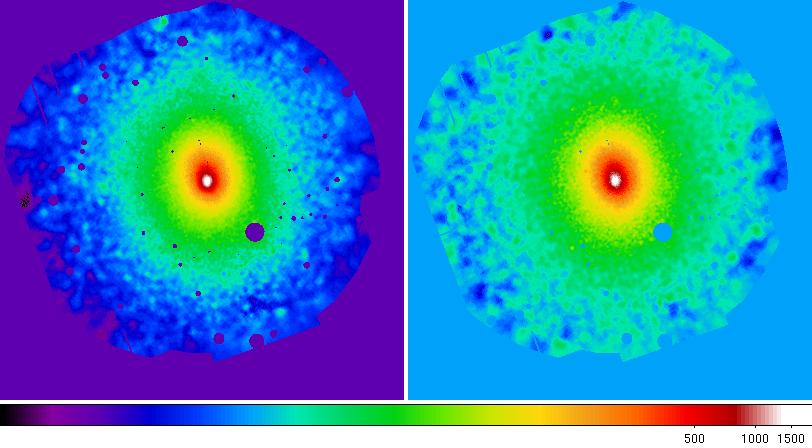
Figure 9: Abell 1795 adaptively smoothed, background subtracted, and exposure corrected images in the 0.4-1.25 keV and 2.0-7.2 keV bands.
- Now, redo the processing to limit the spectrum to the outer annulus. This excludes
the bright cluster emission at the center of the field of view and will produce a better
fit for the SP contamination. In this case this will reduce the fitted amount
of SP contamination. Create the regm1-ann.txt, regm2-ann.txt, and
regpn-ann.txt selection expressions. Note that the regions should cover the same
part of the sky. Since the pn optical axis is offset from the center of the detector so
on-axis sources will not fall in the chip gap, the annulus is smaller than the active areas.
regm1-ann.txt: &&((DETX,DETY) IN circle(134,-219,14200))&&!((DETX,DETY) IN circle(134,-219,10600))
regm2-ann.txt: &&((DETX,DETY) IN circle(6,-93,14200))&&!((DETX,DETY) IN circle(6,-93,10600))
regpn-ann.txt: &&((DETX,DETY) IN circle(59,-10,14200))&&!((DETX,DETY) IN circle(59,-10,10600))Run mos-spectra, pn-spectra, mos_back, and, pn_back to do the spectral extraction and prepare for the background modeling. Use band limits of 0 0 since we aren't interested in recreating the image components.
mos-spectra prefix=1S003 caldb=/PATH/esascaldb region=reg.txt mask=1 \
elow=0 ehigh=0 ccd1=1 ccd2=1 ccd3=1 ccd4=1 ccd5=0 ccd6=1 ccd7=1
mos-spectra prefix=2S004 caldb=/PATH/esascaldb region=reg.txt mask=1 \
elow=0 ehigh=0 ccd1=1 ccd2=1 ccd3=1 ccd4=1 ccd5=1 ccd6=1 ccd7=1
pn-spectra prefix=S005 caldb=/software/XMM/CCF/esas region=pn-reg.txt \
mask=1 elow=0 ehigh=0 pattern=4 quad1=1 quad2=1 quad3=1 quad4=1
mos_back prefix=1S003 caldb=/PATH/esascaldb diag=0 elow=0 ehigh=0 \
ccd1=1 ccd2=1 ccd3=1 ccd4=1 ccd5=0 ccd6=1 ccd7=1
mos_back prefix=2S004 caldb=/PATH/esascaldb diag=0 elow=0 ehigh=0 \
ccd1=1 ccd2=1 ccd3=1 ccd4=1 ccd5=1 ccd6=1 ccd7=1
pn_back prefix=S005 caldb=/PATH/esascaldb diag=0 elow=0 ehigh=0 \
pattern=4 quad1=1 quad2=1 quad3=1 quad4=1
- For convenience, rename a few files so that they are not overwritten.
mv mos1S003-obj.pi mos1S003-obj-ann.pi
mv mos1S003.rmf mos1S003-ann.rmf
mv mos1S003.arf mos1S003-ann.arf
mv mos1S003-back.pi mos1S003-back-ann.pi
mv mos1S003-obj-im-sp-det.fits mos1S003-sp-ann.fits
mv mos2S004-obj.pi mos2S004-obj-ann.pi
mv mos2S004.rmf mos2S004-ann.rmf
mv mos2S004.arf mos2S004-ann.arf
mv mos2S004-back.pi mos2S004-back-ann.pi
mv mos2S004-obj-im-sp-det.fits mos2S004-sp-ann.fits
mv pnS005-obj-os.pi pnS005-obj-os-ann.pi
mv pnS005-obj.pi pnS005-obj-ann.pi
mv pnS005-obj-oot.pi pnS005-obj-oot-ann.pi
mv pnS005.rmf pnS005-ann.rmf
mv pnS005.arf pnS005-ann.arf
mv pnS005-back.pi pnS005-back-ann.pi
mv pnS005-obj-im-sp-det.fits pnS005-sp-ann.fits
- Group the spectral data in preparation for spectral fitting.
specgroup spectrumset=mos1S003-obj-ann.pi mincounts=100 rmfset=mos1S003-ann.rmf \
arfset=mos1S003-ann.arf backgndset=mos1S003-back-ann.pi groupedset=mos1S003-obj-ann-grp.pi
specgroup spectrumset=mos2S004-obj-ann.pi mincounts=100 rmfset=mos2S004-ann.rmf \
arfset=mos2S004-ann.arf backgndset=mos2S004-back-ann.pi groupedset=mos2S004-obj-ann-grp.pi
specgroup spectrumset=pnS005-obj-os-ann.pi mincounts=100 rmfset=pnS005-ann.rmf \
arfset=pnS005-ann.arf backgndset=pnS005-back-ann.pi groupedset=pnS005-obj-os-ann-grp.pi
- Determine the solid angle and fit the data.
proton_scale caldb=/PATH/esascaldb mode=1 detector=1 maskfile=mos1S003-sp-ann.fits \
specfile=mos1S003-obj-ann.pi
proton_scale caldb=/PATH/esascaldb mode=1 detector=2 maskfile=mos2S004-sp-ann.fits \
specfile=mos2S004-obj-ann.pi
proton_scale caldb=/PATH/esascaldb mode=1 detector=2 maskfile=pnS005-sp-ann.fits \
specfile=pnS005-obj-ann.pi
Fit the spectral data to determine the soft proton contamination parameters (Xspec XCM file). Note that the fitting process is complicated with a strong likelihood of local minima. The Al, Si, and Cu fluorescent background lines in particular should start frozen until a reasonably good fit is achieved and then thawed. After a new, and probably a significantly better fit is achieved they can be frozen again to reduce the number of free parameters and again improve the fit.
The result of the annular fitting process is shown if Figure 10. The cluster emission is now relatively minor allowing for a much improved fit to the various background components.
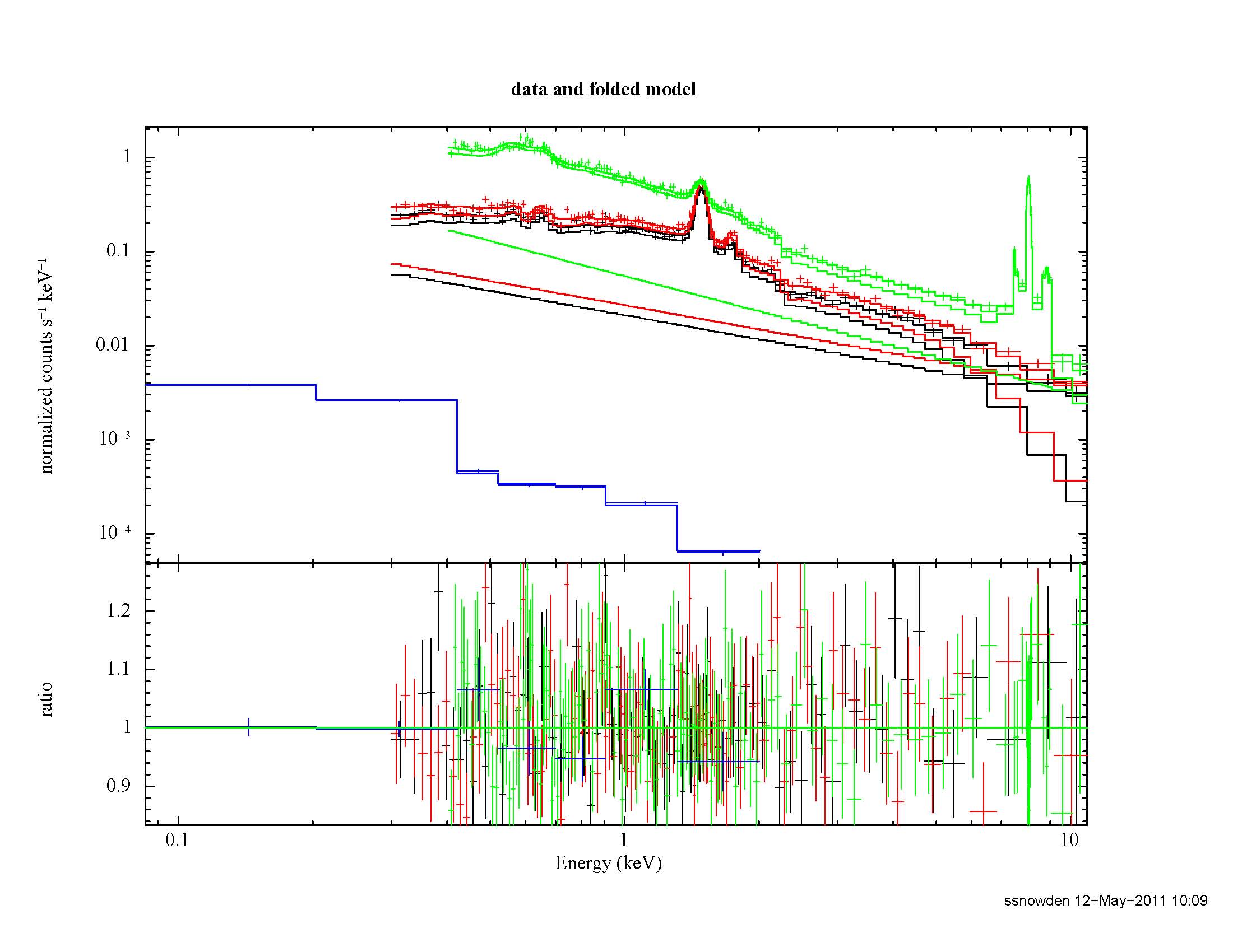
Figure 10: Best fit of the Abell 1795 data from the outer annulus. The green data and model curves are from the pn, the black and red data and model curves are from the MOS1 and MOS2, respectively, and the blue model and curve are from the RASS. The straight line model curves for the MOS and pn are the soft proton contribution.
- Scale the fitted SP results for the limited region to the whole FOV. sp_partial
scales the normalization from one extracted region to that of another, in this case the
full FOV.
sp_partial caldb=/PATH/esascaldb detector=1 fullimage=mos1S003-sp-full.fits \
fullspec=mos1S003-obj-full.pi regionimage=mos1S003-sp-ann.fits \
regionspec=mos1S003-obj-ann.pi rnorm=1.91173E-02
sp_partial caldb=/PATH/esascaldb detector=2 fullimage=mos2S004-sp-full.fits \
fullspec=mos2S004-obj-full.pi regionimage=mos2S004-sp-ann.fits \
regionspec=mos2S004-obj-ann.pi rnorm=2.60037E-02
sp_partial caldb=/PATH/esascaldb detector=3 fullimage=pnS005-sp-full.fits \
fullspec=pnS005-obj-os-full.pi regionimage=pnS005-sp-ann.fits \
regionspec=pnS005-obj-os-ann.pi rnorm=4.17380E-02
- proton
uses the fitted soft proton parameters to create images of
the soft proton contamination in detector coordinates. Use the fitted power law
index from the annular fit.
proton prefix=1S003 caldb=/PATH/esascaldb ccd1=1 ccd2=1 ccd3=1 ccd4=1 ccd5=0 \
ccd6=1 ccd7=1 elow=400 ehigh=1250 spectrumcontrol=1 pindex=0.798623 pnorm=6.6442311E-02
proton prefix=1S003 caldb=/PATH/esascaldb ccd1=1 ccd2=1 ccd3=1 ccd4=1 ccd5=0 \
ccd6=1 ccd7=1 elow=2000 ehigh=7200 spectrumcontrol=1 pindex=0.798623 pnorm=6.6442311E-02
proton prefix=2S004 caldb=/PATH/esascaldb ccd1=1 ccd2=1 ccd3=1 ccd4=1 ccd5=1 \
ccd6=1 ccd7=1 elow=400 ehigh=1250 spectrumcontrol=1 pindex=0.798623 pnorm=8.6460449E-02
proton prefix=2S004 caldb=/PATH/esascaldb ccd1=1 ccd2=1 ccd3=1 ccd4=1 ccd5=1 \
ccd6=1 ccd7=1 elow=2000 ehigh=7200 spectrumcontrol=1 pindex=0.798623 pnorm=8.6460449E-02
proton prefix=S005 caldb=/PATH/esascaldb ccd1=1 ccd2=1 ccd3=1 ccd4=1 \
elow=400 ehigh=1250 spectrumcontrol=1 pindex=1.09442 pnorm=0.1397047
proton prefix=S005 caldb=/PATH/esascaldb ccd1=1 ccd2=1 ccd3=1 ccd4=1 \
elow=2000 ehigh=7200 spectrumcontrol=1 pindex=1.09442 pnorm=0.1397047
- Use rot-im-det-sky
again to rotate the detector coordinate soft proton background
images into sky coordinates.
rot-im-det-sky prefix=1S003 mask=0 elow=400 ehigh=1250 mode=2
rot-im-det-sky prefix=1S003 mask=0 elow=2000 ehigh=7200 mode=2
rot-im-det-sky prefix=2S004 mask=0 elow=400 ehigh=1250 mode=2
rot-im-det-sky prefix=2S004 mask=0 elow=2000 ehigh=7200 mode=2
rot-im-det-sky prefix=S005 mask=0 elow=400 ehigh=1250 mode=2
rot-im-det-sky prefix=S005 mask=0 elow=2000 ehigh=7200 mode=2
- comb
combines the MOS1, MOS2, and pn images, as well as images from multiple
exposures. Since the spectra and images were created with point sources
removed comb
must be run using the cheese masking.
comb caldb=/software/XMM/CCF/esas withpartcontrol=1 withsoftcontrol=1 withswcxcontrol=0 \
nbands=1 elowlist=400 ehighlist=1250 mask=1 ndata=3 prefixlist="1S003 2S004 S005"
comb caldb=/software/XMM/CCF/esas withpartcontrol=1 withsoftcontrol=1 withswcxcontrol=0 \
nbands=1 elowlist=2000 ehighlist=7200 mask=1 ndata=3 prefixlist="1S003 2S004 S005"
- Adaptively smooth the images.
adapt_900 smoothingcounts=50 thresholdmasking=0.02 detector=0 binning=2 elow=400 ehigh=1250 \
withpartcontrol=yes withsoftcontrol=yes withswcxcontrol=0
adapt_900 smoothingcounts=50 thresholdmasking=0.02 detector=0 binning=2 elow=2000 ehigh=7200 \
withpartcontrol=yes withsoftcontrol=yes withswcxcontrol=0
- Rename and display the smoothed images.
mv adapt-400-1250.fits adapt-400-1250-ann.fits
mv adapt-2000-7200.fits adapt-2000-7200-ann.fits
ds9 adapt-400-1250-ann.fits adapt-2000-7200-ann.fits
Figure 11 shows the final adaptively smoothed, background subtracted, and exposure corrected images, this time with the better parametrization of the background components allowed by using the outer annulus. The effect is most clearly shown in the 0.4-1.25 keV band where the background is no longer over-subtracted.
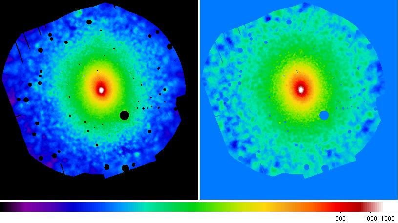
Figure 11: Abell 1795 adaptively smoothed, background subtracted, and exposure corrected images in the 0.4-1.25 keV and 2.0-7.2 keV bands.
- If necessary (not in this observation) the task swcx can be used to
model the contribution of SWCX to the image to be subtracted. swcx uses
the fitted values for SWCX lines fluxes to model their image contributions.
swcx prefix=1S003 caldb=/software/XMM/CCF/esas ccd1=1 ccd2=1 ccd3=1 ccd4=1 ccd5=0 ccd6=1 ccd7=1 \
elow=400 ehigh=1250 linelist='1 2' gnormlist='0.0 7.65634E-08' objarf=mos1S003-full.arf \
objspec=mos1S003-obj-full.pi
swcx prefix=2S004 caldb=/software/XMM/CCF/esas ccd1=1 ccd2=1 ccd3=1 ccd4=1 ccd5=1 ccd6=1 ccd7=1 \
elow=400 ehigh=1250 linelist='1 2' gnormlist='0.0 7.65634E-08' objarf=mos2S004-full.arf \
objspec=mos2S004-obj-full.pi
swcx prefix=S005 caldb=/software/XMM/CCF/esas ccd1=1 ccd2=1 ccd3=1 ccd4=1 elow=400 ehigh=1250 \
linelist='1 2' gnormlist='0.0 7.65634E-08' objarf=pnS005-full.arf objspec=pnS005-obj-full.pi
- SWCX images are also created in detector coordinates and so must be rotated into sky
coordinates.
rot-im-det-sky prefix=1S003 mask=0 elow=400 ehigh=1250 mode=3
rot-im-det-sky prefix=2S004 mask=0 elow=400 ehigh=1250 mode=3
rot-im-det-sky prefix=S005 mask=0 elow=400 ehigh=1250 mode=3
- comb combines the MOS1, MOS2, and pn images, as well as images from multiple
exposures. Since the spectra and images were created with point sources
removed comb must be run using the cheese masking.
comb caldb=/software/XMM/CCF/esas withpartcontrol=1 withsoftcontrol=1 withswcxcontrol=1 \
nbands=1 elowlist=400 ehighlist=1250 mask=1 ndata=3 prefixlist="1S003 2S004 S005"
comb caldb=/software/XMM/CCF/esas withpartcontrol=1 withsoftcontrol=1 withswcxcontrol=1 \
nbands=1 elowlist=2000 ehighlist=7200 mask=1 ndata=3 prefixlist="1S003 2S004 S005"
- Adaptively smooth the images.
adapt_900 smoothingcounts=50 thresholdmasking=0.02 detector=0 binning=2 elow=400 ehigh=1250 \
withpartcontrol=yes withsoftcontrol=yes withswcxcontrol=0
adapt_900 smoothingcounts=50 thresholdmasking=0.02 detector=0 binning=2 elow=2000 ehigh=7200 \
withpartcontrol=yes withsoftcontrol=yes withswcxcontrol=0
- Rename and display the smoothed images.
mv adapt-400-1250.fits adapt-400-1250-ann-swcx.fits
mv adapt-2000-7200.fits adapt-2000-7200-ann-swcx.fits
ds9 adapt-400-1250-ann-swcx.fits adapt-2000-7200-ann-swcx.fits
Last Updated: 10 May 2011
|
Caveats
For information about known issues, refer to the ESAS Warnings and Watchouts pages. |
Download the Adobe Acrobat (PDF) Reader.
If you have any questions concerning XMM-Newton send email to xmmhelp@athena.gsfc.nasa.gov
