4. X-Ray Mirror Assembly (XMA)

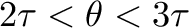
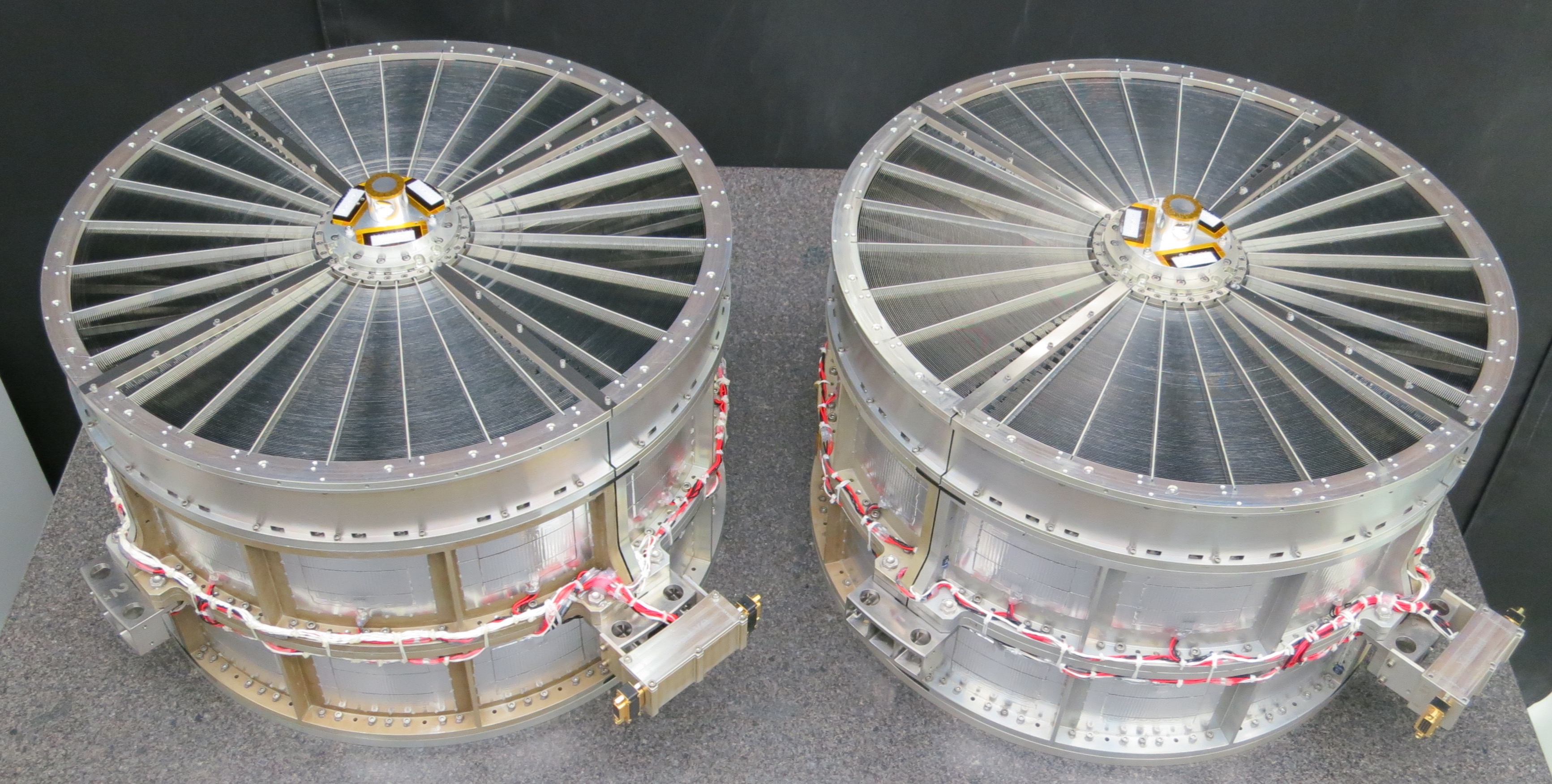
XRISM has two X-ray Mirror Assemblies (XMAs) focusing X-rays onto the focal plane detectors. One of these mirrors, Resolve-XMA, focuses X-rays on Resolve, while the other, Xtend-XMA, is used with Xtend. Both mirrors have identical design and improve on the mirrors on-board Suzaku. The entire system (see Figure 4.1) consists of an X-ray mirror, a Pre-Collimator (PC) stray light baffle, and a thermal shield.

Figure 4.1: Image of the XMA with all its components.

Figure 4.2: Picture of the X-ray Mirror Assemblies, without thermal shields (right: Resolve-XMA, left: Xtend-XMA).

Table 4.1: XMA parameters and their characteristics.

	XRISM XMA
Focal length	5.6 m
Effective aperture diameter	12 – 45 cm
Height	20 cm
Number of reflectors	203
Reflecting surface	gold
Grazing angle	0.15$^\circ$ – 0.57$^\circ$
Energy range$^1$	0.3 – 15 keV
Effective Area$^2$	587  cm$^2$ 1.5 keV
	438  cm$^2$ 4.5 keV
	418  cm$^2$ 6.4 keV
Angular Resolution (HPD)	1.3$^\prime$ for Resolve-XMA and 1.5$^\prime$ for Xtend-XMA
Angular Resolution (FWHM)	8 $^{\prime\prime}$ for Resolve-XMA and 7 $^{\prime\prime}$ for Xtend-XMA
$^1$The nominal energy range of XMAs is 0.3 – 15 keV. XMAs have sensitivity to higher energy ($>15$ keV) photons but the calibration accuracy declines. $^2$Includes telescope, pre-collimator, thermal shield but not the detectors. Values are from Boissay-Malaquin et al. (2022).

4.1 XMA Components

4.1.1 Mirror Part

The XMA mirror, with an outer diameter of 45 cm, and a 5.6 m focal length, uses conical approximations to the Wolter Type I configuration with 203 nested shells consisting of 1624 individual reflectors (Figure 4.2). The reflective surfaces of the reflectors consist of a single-layer coating of gold. The reflectors are arranged in four quadrants for each set of primary and secondary housings. Seven holding bars on the top and bottom sides support the reflectors. The reflector substrates are composed of Aluminum, and the 203 shells are organized into three groups, with different substrates thicknesses per group. An epoxy buffer layer helps focus grazing-incidence X-rays with energies up to 15 keV. In addition to the reflectors, bare substrate foils are installed inside the innermost primary reflectors to stop the incident X-rays from directly arriving at the innermost secondary which is a path producing the stray light (see Section 4.1.2). A pre-collimator, installed for stray light protection, consist of coaxially nested cylindrical aluminum blades placed above each reflector. A thermal shield (TS) is attached in front of the pre-collimator to stabilize the thermal environment of the XMAs. The shield is made of Al-coated Polyimide to ensure a large effective area in the soft energy band. The thermal shield transmits soft X-rays but helps to reduce the radiative heat transfer into and out of each XMA.

The final result is a relatively light mirror with large throughput over a broad energy range (Serlemitsos et al., 2010, and references therein). Although largely inspired by Suzaku's mirrors, the two XMA mirrors benefited from both relaxed weight constraints and several fabrication improvements, including thicker substrates, a larger number of forming mandrels, thinner epoxy layer for replication, stiffer housings, and higher-precision alignment. All these improvements yield better overall mirror performances, including a smaller angular resolution and an improved effective area both at 1 keV and at 6 keV (Okajima et al., 2012). The XMA was developed at NASA GSFC in collaboration with JAXA/ISAS, and Tokyo Metropolitan University in Japan. The summary of each mirror performance compared when necessary to the relevant requirement is given in Table 4.1. Unless explicitly noted, the parameters mentioned in the table are identical for both mirrors.

4.1.2 Pre-Collimator

Figure 4.3: Major reflection paths occurring in the XMA structure. (a) Normal double reflection of the X-ray arriving from the on-axis direction. Incident X-rays are bent by the angle 4$\tau$ in total, and converge to the on-axis focus: (b) Secondary reflection, which arrives at the focal plane only if the incident angle of the X-ray, $\theta$, measured from the optical axis is in the range $\tau < \theta <2 \tau$: (c) Stray light path that gives rise to the brightest ghost among various backside reflections, the reflection at the backside of the primary followed by the normal double reflection. This pattern occurs when the X-ray incident angle is in the range $2\tau < \theta <3 \tau$. From Mori et al. (2005).

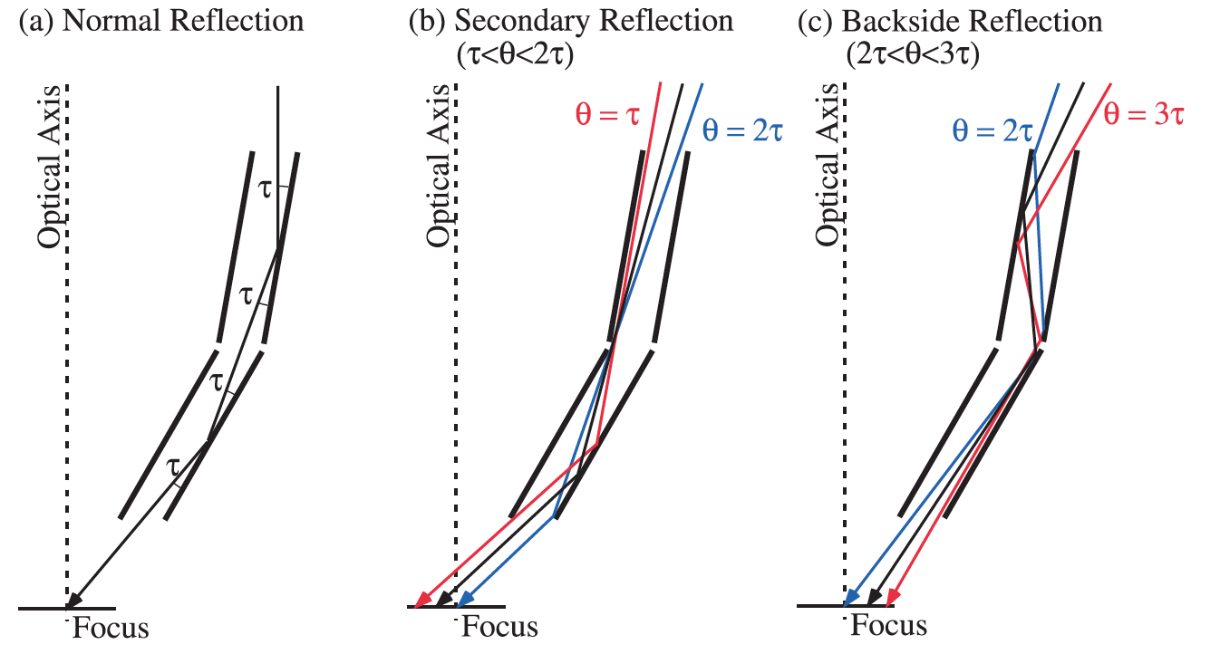
The grazing-incidence optics adopted for X-ray imagining use a large number (203 in the case of XRISM) of reflectors nested as tightly as possible to increase the effective area. As a result, this configuration increases the possibility of reflection other than the normal double reflection within the telescope. These contaminations of abnormal paths are referred to as “stray light." Studies on the ASCA stray light (Mori et al., 2005) showed that the main contribution to the stray light is from secondary reflections of photons with an incident angle between $\tau$ and 2$\tau$ (where $\tau$ is the angle of the primary reflector measured from the optical axis of the telescope – see Figure 4.3). Therefore, a pre-collimator is installed in order to address the issue of both secondary and backside reflection that would otherwise contaminate data on the focal plane.

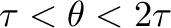
The Pre-Collimator (PC) built for XRISM is derived from the one on Suzaku. Each PC consists of cylindrical aluminum shells (blades) with varying radii of 60 – 225 mm, alignment frames to guide the blade positions, and the blade housing body. Each PC blade is placed precisely on top of the respective reflector to reduce off-axis X-ray photons that leads to a “ghost" image within the detector field of view. Since the secondary reflection is caused by the off-axis X-rays going just above the primary mirrors, these cylindrical blades can block this component effectively. The blade thickness is designed to be narrower than that of the reflector. Thus, there is no loss of the on-axis effective area if the alignment between the mirrors and blades is attained. The alignment frame and the housing are made of Aluminum. Heat-forming process is introduced to the production to stabilize the blade shape in orbit. Precise curvature of radius and the linearity along with the direction of incident X-rays ensure that the blades do not obscure the telescope aperture. Figure 4.4 shows a pre-collimator and its geometry and Table 4.2 shows the main characteristics of the XMA pre-collimator.

Table 4.2: The main characteristics of the XMA pre-collimator.

Number of segments	4
Material	Aluminum
Number of blades	204
Number of support bars	7

Figure 4.4: Image of a Pre-collimator quadrant used for XRISM XMA.

Figure 4.5: Image of a thermal shield quadrant used for XRISM XMA.

4.1.3 Thermal shields and heaters

Per requirement, the operating temperature of the telescopes in orbit must be maintained at 22 $^\circ \pm$ 7 $^\circ$C. This is achieved by covering the entrance side with a thermal shield (TS) composed of the 4 thermal shield quadrants shown in Figure 4.5 for each XMA. These shields isolate the telescopes thermally from space and reflect infrared radiation from the interior of the spacecraft. The thermal shields also work to block optical light coming either from the sky or from the surface of Earth illuminated by the Sun.

The shields are made of an aluminized Polyimide glued to a supporting stainless-steel mesh. The reflectivity in the optical wave band is more than 90%, and yields a rejection of the optical light from the bright Earth and the reflection of the IR radiation from the telescopes at $\sim$290 K back to the interior of the satellite. In addition to the shields, heaters are affixed to the wall of the housing to keep it within the mandated temperature range. The whole XMAs are inside the sunshade base. Thermometers are attached to the wall to monitor the temperature and control the heaters.

4.2 Expected Performance

4.2.1 Focal Positions and Optical Axis

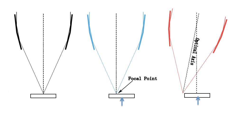
For each mirror, the transmission is maximized when the target is observed along the optical axis. The left diagram of Figure 4.6 shows the “ideal" telescope+detector system. The actual configuration of a mirror includes a shift between the focal point and the detector aimpoint (shown in the middle diagram) and a tilt of the mirror optical axis with respect to the nominal aim-point (shown in the right diagram). Moving off the detector aimpoint from the mirror on-axis focal point results in reducing the effective area due to vignetting. This places the boresight measurement and the determination of the optical axis position as one of the highest priority among the calibration requirements for both instruments. The detector aim point is defined as the center of the Rosolve field of view. The optical axis is tilted about 15" with respect to the nominal aim-point direction, as this angle makes the maximum on-axis effective area. With this small angle, the loss of the effective area is less than 0.5% due to vignetting and is negligible. However, the focal point may shift to +Y direction as indicated in Figure 4.7. Xtend is on-axis at aim point (less than 3" shift). Detailed in-flight calibration is forthcoming. However, the alignment configuration measured at the ground should be adequate for Cycle 1 proposal preparation. Figure 4.7 indicates the location of the detector aim point with respect to the Xtend and Resolve FoVs. The boresight and the pointing accuracy are around 20 arcsec for Resolve and Xtend.

Figure 4.6: Cartoon view of the actual configuration of a mirror compared to the ideal geometry (shown on the left). The middle picture illustrates the shift between the focal point and the detector aim point and the right picture shows in addition the effect of a tilt of the optical axis with respect to the nominal aim-point direction (HITOMI in-flight calibration plan, 2015.)

Figure 4.7: Left: Layout of Xtend FoV (black) superimposed with Resolve FoV (cyan). This is a look-up view. The expected Xtend aimpoint is located from $\sim$5.0$^\prime$ (DETX) and $\sim$ 5.4$^\prime$ (DETY) from the edges of the CCD. The ground calibration reported that Xtend is on-axis at aim point (less than 3" shift). Right: The expected aimpoint of Resolve as the center of Resolve FoV. The ground calibration reported that optical axis of the XMA-Resolve is slightly shifted. In-flight calibration is on-going.

4.2.2 Effective Areas

The predicted effective area of both the Xtend-XMA and Resolve-XMA can be calculated using ground measurements combined with ray-tracing simulations. Table 4.3 lists the ground measurements for both the Xtend-XMA and Resolve-XMA (Boissay-Malaquin et al., 2022). The simulated effective area curves are plotted in Figure 4.8.

Table 4.3: Effective area (in cm$^2$) for both XMAs (with 68% statistical errors), at different energies E, for the whole telescope axis. From Boissay-Malaquin et al. (2022)

Energy [keV]	Effective Area (cm$^2$)
	Resolve-XMA	Xtend-XMA
1.5	584.7 $\pm$ 0.4	589.4 $\pm$ 0.4
4.5	434.7 $\pm$ 0.6	441.5 $\pm$ 0.6
6.4	416.0 $\pm$ 0.6	422.2 $\pm$ 0.6
8.0	345.3 $\pm$ 0.8	349.2 $\pm$ 0.8
9.4	233.4 $\pm$ 0.6	235.5 $\pm$ 0.6
11.0	163.4 $\pm$ 0.4	164.5 $\pm$ 0.4
17.5	38.4 $\pm$ 0.2	37.9 $\pm$ 0.1

Figure 4.8: Effective area versus energy, for Xtend-XMA (black) and Resolve-XMA (red) plotted on the linear scale (left) and on the log scale (right). Note that these simulated curves are based on ground measurements and the XMA-only effective areas, thus not including QE of the detectors, etc..

4.2.3 Vignetting

The vignetting measures the variation of the effective area as a function of off-axis angle. It also depends on the photon energy as well as the azimuthal angle. The left panel of Figure 4.9 shows the vignetting curves measured on the ground at different energies (shown by open squares on the plot) fitted with 1D Lorentzian model, for Cross direction 1 (azimuthal angle: 0-180$^\circ$, see the right panel of Figure 4.9), for Xtend-XMA. The similar curves for Resolve-XMA is shown in Figure 4.10, using a smaller off-axis angle range and 1D Lorentzian model. Figure 4.11 shows these vignetting curves at 6.4 keV for 8 different azimuthal angles for both well fitted with Resolve-XMA and Xtend-XMA, revealing a very similar mirror FoV (defined as FWHM at 6.4 keV of 1D Lorentzian model) of about 14 arcmin for both XMAs.

Figure 4.12 shows the size of XMAs' Field of View (not the detector FoVs), as a function of energy.

Figure 4.9: Left: Vignetting curves of all energies, for Xtend-XMA, for azimuthal 0-180 deg, fitted with the sum of Lorentzian and Gaussian models to the data measured on the ground. Right: Look-down illustration of the mirror roll angle (different from the spacecraft roll angle) and the off-axis angle used during the ground calibration measurements (see Boissay-Malaquin et al. (2022)). The coordinates of the satellite and detector are shown, as well as the boundaries of the XMAs’ quadrants.

Figure 4.10: Vignetting curves of all energies, for Resolve-XMA, for roll angle (azimuthal angle) 0-180 deg, fitted with 1D Lorentzian model fitted to the data measured on the ground.

Figure 4.11: Vignetting curves at 6.4 keV fitted to the data points measured on the ground, for Resolve-XMA (left) and Xtend-XMA (right), for 8 roll (azimuthal) angles (see the right panel of Figure 4.9).

Figure 4.12: Field of View of the XMAs, as a function of energy. The FoV is defined here as the FWHM value determined by fitting the vignetting curves with a 1D Lorentzian model, and does not take the physical size of the detectors into account. The FoV is the average value of the FWHM in all directions. The data points are from the ground measurements.

4.2.4 Angular Resolution

The Point-Spread Function (PSF) was measured at nine different energies. Figure 4.13 shows the on-axis focal plane image of the Resolve-XMA and Xtend-XMA, illustrating that the PSF has structures. The PSF structures may have to be taken into account when planning to observe a bright source or analyzing extended sources with a bright point source (Chapters 7 and 8). One-dimensional PSF, which was normalized so that the total number of photons is unity within a radius of 8$^\prime$, and of the Encircled Energy Function (EEF) for both Xtend-XMA and Resolve-XMA are given in Figure 4.14 and Figure 4.15, respectively. Both figures also exhibit that the profiles are a function of the incoming photon energy. Table 4.4 summarizes the values of the Half-Power Diameter (HPD) angular resolution. For both mirrors, the measured HPD is found to be better than the 1.7$^\prime$ requirement (Tamura et al., 2022). The typical error of the angular resolution is about 0.01$^\prime$ in HPD, based on statistical error, uncertainty in the position of the center of the image, and the fluctuation of the CCD background. The angular resolution of the Resolve-XMA is about 0.1$^\prime$-0.2$^\prime$ better than that of Xtend-XMA at all energies.

Table 4.4: The HPD obtained at seven energies. From Tamura et al. (2022)

Energy [keV]	1.49	4.50	6.40	8.05	9.44	11.07	17.48
Resolve-XMA [$^\prime$]	1.29	1.30	1.30	1.28	1.22	1.19	1.24
Xtend-XMA [$^\prime$]	1.47	1.46	1.47	1.47	1.40	1.37	1.37

Figure 4.13: Focal plane images of Resolve-XMA (top) and Xtend-XMA (bottom) at the six energies of 1.49, 4.50, 6.40, 8.05, 9.44, and 11.07 keV (Tamura et al., 2022). The image size is 6.7$^\prime$ $\times$ 6.7$^\prime$.

Figure 4.14: One-dimensional PSFs of Resolve-XMA (left) and Xtend-XMA (right). The six PSFs at 1.49 (red), 4.50 (green), 6.40 (blue), 8.05 (light blue), 9.44(violet), and 11.07 keV (dark blue) are plotted (Tamura et al., 2022). These plots are based on the ground measurements.

Figure 4.15: The EEF of the Resolve-XMA (left) and the Xtend-XMA (right). The six EEFs at 1.49 (red), 4.50 (green), 6.40 (blue), 8.05 (light blue), 9.44 (violet), and 11.07 (dark blue) are plotted (Tamura et al., 2022). These plots are based on the ground measurements.

4.2.5 Stray Light

Stray light designates X-rays that enter the detector via a path other than the normal double reflections. It includes the case of a single reflection on either reflector, a reflection on the back side of the reflectors, or a reflection on the pre-collimator blade. The pre-collimator significantly reduces the amount of stray light (as seen in 4.1.2), but it also causes slight stray light. Stray light that can occur in a multi-nested thin foil optic was discussed in detail by Mori et al. (2005). Figure 4.16 shows the stray light images at 1.49 keV obtained at 30$^\prime$ and 60$^\prime$ off-axis angles at an azimuthal angle. In both images, the X-ray source is positioned on the right side. This is the same stray light structure reported for the Hitomi SXT mirrors (Iizuka et al., 2018). The 30$^\prime$ off-axis image has a component biased to the right side of the image, while in the 60$^\prime$ off-axis image there is stray light spread over the entire detector. The stray light seen on the right side of the 30$^\prime$ off-axis images is due to the reflection of the pre-collimator, while the extended component is mainly due to the reflection on the backs of the reflectors. We note that the direct component coming through the gap between the inner wall of the housing and the innermost reflector reported for Hitomi SXT Mirror (Iizuka et al., 2018) is not seen in XMAs, because bare aluminum foil was added inside the innermost reflector to removes the direct incident component (Tamura et al., 2022). The main contributions on the measured stray light for XMAs are probably due to pre-collimator reflections. The amount of stray light entering within an 8$^\prime$ radius, converted to effective area, is shown in Table 4.5 as well as the amount of stray light entering the Resolve detector. We note that the flux of the stray depends on the azimuthal direction of the incident photons, and the values in Table 4.5 are instances. The detailed analysis of stray light will be performed with the in-flight calibration data. However, expected stray light effects will not be large based on Suzaku observations. Therefore, proposers are not expected to consider stray light contamination on their targets when planning proposal submissions.

Table 4.5: The effective area at 1.49 keV for off-axis sources due to stray light. From Tamura et al. (2022)

	Resolve-XMA (r$<$8$^\prime$)	Resolve-XMA (Reslove FoV)	Xtend-XMA (r$<$8$^\prime$)
30$^\prime$ off-axis [cm$^2$]	0.26 $\pm$ 0.01	0.007 $\pm$ 0.001	0.16 $\pm$ 0.01
60$^\prime$ off-axis [cm$^2$]	0.18 $\pm$ 0.01	0.009 $\pm$ 0.001	0.11 $\pm$ 0.01

Figure 4.16: Stray light images of Resolve-XMA (top) and Xtend-XMA (bottom) at 30$^\prime$ off axis angle (left) and 60$^\prime$ off axis (right) (Tamura et al., 2022). The X-ray energy is 1.49 keV. The image size is 17.8$^\prime$ $\times$17.8$^\prime$. The FOV of Resolve is shown in left top panel.