5. Resolve

Resolve is a high resolution X-ray imaging spectrometer with a $3' \times 3'$ field-of-view. It consists of X-ray focusing mirrors (XMA, Chapter 4), and a 36-pixel X-ray calorimeter system (XCS) with better than 5 eV resolution over much of the 1.7-12 keV energy band, according to the initial in-orbit calibration. An anti-coincidence detector placed behind the calorimeter array enables rejection of particle background events.

Key performance parameters are provided in Table 5.1 and an overall view of the Resolve is shown in Figure 5.1. Figure 5.2 shows the effective area of the instrument. The nominal energy range of Resolve is 1.7-12 keV. At low energies, the effective area of Resolve declines steeply due to the closed gate valve ($\sim$0.5 cm$^2$ at 1.7 keV). At high energies, Resolve is sensitive to photons above 12 keV, even up to $\sim$20 keV. However, calibration becomes less reliable at high energies, and 12 keV is currently the high end of the nominal Resolve energy range.

Table 5.1: Summary of the expected Resolve detector properties based on the ground calibration. HPD stands for Half Power Diameter.

Parameter	Expected
Lifetime	Goal: 5 years
Energy range	1.7-12 keV
Effective area	$\sim$ 180 cm$^2$ @6keV
Angular resolution	1.3$'$ HPD
Energy resolution	5 eV (FWHM)
Energy-scale accuracy	0.5 eV
Line-spread function accuracy	Goal: 1 eV
Pixel size	30”$\times$30”
	818 $\mu$m$\times$ 818 $\mu$m
Field of View	$3.1'\times 3.1'$
Array format	$6\times6$
	35 science pixels
	1 calibration pixel
Relative timing accuracy	80 $\mu$s for high- and mid-res events
Operating temperature	50 mK
Maximum X-ray count rate	200 counts s$^{-1}$ array$^{-1}$
Residual background	0.8 $\times$ 10$^{-3}$ counts s$^{-1}$ keV$^{-1}$

Figure 5.1: A schematic of the Resolve microcalorimeter array focal plane. Dimensions shown are the design values, but most actual absorbers were 0.818 mm wide, and the gaps were correspondingly smaller on average.

Figure 5.2: Effective area of Resolve, which includes the gate valve transmission (Midooka et al., 2021).

Resolve is descended from the X-ray Spectrometer onboard Suzaku Observatory (Kelley et al., 2007) and the Soft X-ray Spectrometer (SXS) onboard Hitomi (Kelley et al., 2016). It is the first microcalorimeter detector that is available to guest observers.

5.1 Overview

Figure 2.2 shows the schematic of the position of the Resolve within the satellite. X-rays emerging from the X-ray Mirror Assembly (XMA; see Chapter 4) pass through a Filter Wheel Mechanism (FWM; cf. Section 5.8.1) mounted 91.5 cm from the detector. The FWM has six filter positions: two open, one with $^{55}$Fe calibration source, two for X-ray attenuation to reduce the flux incident on the detector, and one with a polyimide filter. Not all filters are available to observers (cf. Section 5.8.1). Modulated X-ray Sources (MXS; cf. Section 5.6), mounted on the filter wheel axis beyond the FWM with respect to the path of X-rays, serve to calibrate the detector gain. The filter wheel position is user-selectable, while MXS is not.

Beyond the FWM, the X-rays go through the aperture door (i.e. the closed gate valve) and then enter the dewar (a cryogenic vacuum vessel where the microcalorimeter array and anti-coincidence detector reside) through five thin-film filters, each staged at a different temperature, before reaching the detectors. These filters help isolate the cooling system from the ambient environment and attenuate the flux of IR photons (thermal radiation from warmer structures) and UV/optical photons (from the sky) that reach the detector. The optical blocking filters in the dewar are fixed in place. The transmission curve for the full five-filter stack is shown in Figure 5.3.

Figure 5.3: Transmission curve for the non-selectable five-filter blocking filter stack.

The microcalorimeter detector array, along with the anti-coincidence detector, is housed within the Detector Assembly and maintained at its operating temperature of 50 mK by a multi-stage cooling system with a temperature stability better than 2.5 $\mu$K, and with efficiency $>$95% for more than three years. This low operating temperature and its stability enables the detector to attain its required energy resolution. The cooling system is designed with redundant features to be tolerant to some failure cases and to enable operation of the detector beyond the nominal three-year lifetime.

Analog signals from the Detector Assembly are amplified and digitized. The digitized signal is sent to the Pulse Shape Processor (PSP), which detects X-ray events from the data stream and applies an optimal filtering algorithm to determine the pulse heights of X-ray events. Details of PSP are provided in Section 5.3.1.

The microcalorimeter detector does not trigger on optical events, but is sensitive to optical photons. The absorbed energy contributes to noise, thus degrading the X-ray energy resolution. However, photons outside of the passband are highly attenuated by the filter stack, and further by the currently closed aperture door (gate valve), and therefore this effect should not be important.

5.2 The microcalorimeter

The Resolve detects and measures X-rays with a $6\times6$ pixels X-ray microcalorimeter array (see Figure 5.1). There are 35 active pixels in the main array and 36 readout channels. One corner pixel is not wired and, instead, a calibration pixel out of the field of view used with a continuous, collimated $^{55}$Fe source to provide one source of gain tracking for the main array. This pixel is active at all times and is designated as pixel number 12 (in lieu of the inactive corner pixel; cf. Figure 5.1 and Section 5.6).

The pixels are arrayed on a 0.83 mm pitch with a filling factor greater than 96%. Each pixel projects to $0.5'\times0.5'$ on the sky and the entire X-ray sensitive portion of the array subtends a solid angle of $3.05' \times 3.05'$. It is very important to note that these pixels are smaller than the PSF ($0.5'$ pixel vs $1.3'$ HPD). This means that if there are bright sources in and around the FOV or the source is extended, photons from other regions of the sky will scatter into an individual pixel. For more information, see Chapters 7 and 8.

A microcalorimeter detects X-rays using a high-sensitivity thermometer that measures the heat produced by thermalization of photon energy when a photon is absorbed by a low heat capacity absorber.

Since the amplitude of the signal translates into X-ray energy, a microcalorimeter is a single photon detector that measures the energy of every incident photon. By combining 36 independent microcalorimeters in a 6$\times$6 array configuration, the Resolve instrument provides high-energy resolution imaging spectroscopy of point-like and diffuse celestial X-ray sources without the use of dispersive optics Mitsuda et al. (2014,2010), in contrast to the grating instruments on board of XMM-Newton and Chandra. Unprecedented energy resolution is attained at $E>2$ keV (including the Fe K band) for all sources, and at all energies for extended, diffuse sources such as supernova remnants and galaxy clusters.

5.2.1 Photon detection

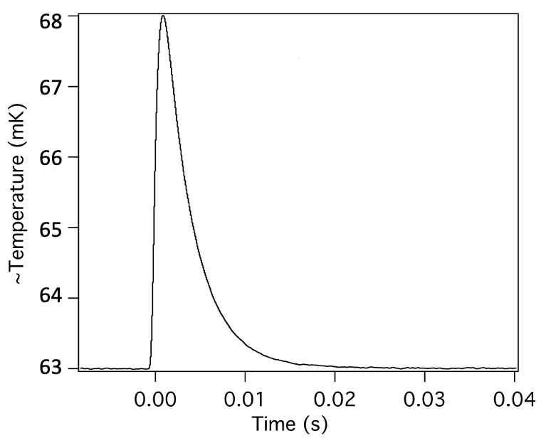
The concept underlying an X-ray quantum microcalorimeter detector is based on the measurement of the temperature increase of an isolated thermal mass. The measurement is made using a thermometer in a quasi-static equilibrium with the absorber (Figure 5.4). Thus, the three essential components are (i) an absorber that absorbs the incident X-ray and thermalizes the deposited energy, (ii) a coupled thermometer that measures the temperature increase in the absorber, and (iii) a weak link to a heat sink that restores the absorber to its original temperature. The energy resolution is determined by the precision of the temperature increase measurement against a background of temperature fluctuations.

For an absorber heat capacity $C_\mathrm{pix}$, thermal link conductance $G_\mathrm{link}$, and heat sink temperature $T_\mathrm{sink}$ the absorber temperature increases by $\Delta T_\mathrm{pix}\approx E_\mathrm{X-ray}/C_{pix}$ (on the order of a $\sim$mK for Resolve) upon absorption of energy $E_\mathrm{X-ray}$ and re-equilibrates to its quiescent temperature with a decay time constant $t_\mathrm{decay}\approx C_\mathrm{pix}/G_\mathrm{link}$. This is illustrated in Figure 5.4.

Figure 5.4: The concept of an X-ray calorimeter is shown in the left panel, whereby an X-ray deposits energy in an absorber that is measured by a thermometer after the energy thermalizes. Subsequently, the absorber returns to its quiescent temperature and the system is ready to detect and measure the next X-ray. Right panel shows a schematic of the temperature of an absorber, which is a part of Resolve pixels, as a function of time. Upon absorbing the photon, the temperature goes up proportionally to the energy of the incident photon, and then goes down with time constant proportional to the heat capacity and thermal link conductivity.

For Resolve, the rise time for the temperature pulse induced by absorption of an X-ray is on the order of a ms, and $t_\mathrm{decay}$ is a few ms. However, the detector requires multiple decay timescales to fully re-equilibrate so that for sufficiently bright sources a second pulse may arrive on the tail of a previous pulse. This is explained further in Section 5.3.3.

5.2.2 Anti-coincidence detector and particle background

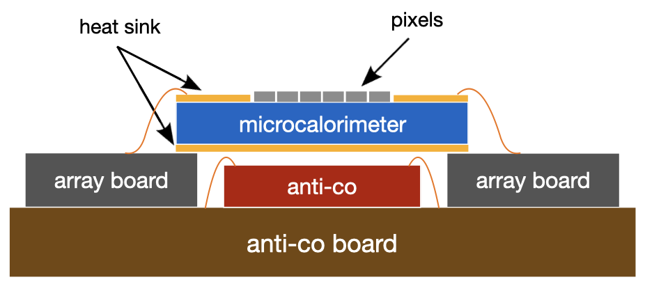
Resolve is equipped with an anti-coincidence (anti-co) detector. Its main purpose is to reject cosmic-ray events that could be incorrectly interpreted as X-rays. Unlike X-ray photons (which are detected by the microcalorimeter only), cosmic rays trigger events in both the microcalorimeter and the anti-co, and thus they can be identified and removed. Additionally, the anti-co provides an independent monitor of the particle environment. In addition to the advantage of the spacecraft being placed in a low-Earth orbit, a lower and more stable particle background compared to other X-ray missions is achieved thanks to the anti-co.

The Resolve anti-co detector is essentially identical to that deployed in SXS on Hitomi (Kilbourne et al., 2018b). It is located directly below the microcalorimeter array, as shown in Figure 5.5. As ionizing charged particles pass through the anti-co, unbound electron/hole pairs are liberated and their drift under the influence of an electric field creates a current that is amplified and measured. Calorimeter events that arise from ionizing particles are flagged for subsequent vetoing as they also trigger a pulse in the anti-co detector. This way the anti-co detector reduces the non X-ray background.

Figure 5.5: Schematic arrangement of the XRISM Resolve microcalorimeter array and the anti-coincidence detector (c.f. Porter et al., 2010). The microcalorimeter array sits on top of the anti-co detector.

The anti-co incidence rejection (i.e., removal of cosmic-ray events) is performed on the ground as part of pipeline processing, allowing for more flexibility in applying different veto timing windows, as well as the capability to conduct spectroscopic analysis of anti-co events.

5.3 Event processing system

5.3.1 Event triggering

Signals from both the microcalorimeter and the anti-co detector are transferred from the Detector Assembly to the XBOX (X-ray amplifier BOX), where they are shaped (via analog high-pass and low-pass filters), amplified, and digitized. The digitized signals are sent to the Pulse Shape Processor (PSP) for event discrimination, classification, and processing. The PSP triggers on pulse candidates and characterizes them, calculating the pulse heights, arrival times, and other characteristics of each event.

A temperature increase in the microcalorimeter due to absorption of an X-ray leads to a drop in resistance and corresponding drop in voltage across the thermistor. The processing results in a profile where peaks are followed by deep, long undershoots that are a result of AC-coupling in the electronics. When the calculated derivative of this amplitude profile exceeds the threshold, an X-ray event is triggered. The characteristic profile of the amplitude of this drop after shaping and inversion in the XBOX is shown in Figure 5.6.

Figure 5.6: Typical shape of a pulse triggered by an incident X-ray. Left panel shows a single photon, while right panel shows a situation where second photon is detected before the pixel equilibrates after the first event. The undershoot following the pulse happens because the electronics are AC coupled. For details, see Section 5.3.1.

The PSP calculates a running boxcar derivative of the incoming data stream of each calorimeter channel, and when that derivative exceeds the selected threshold, an X-ray event is provisionally triggered. Then, a search for events occurring after the first event is conducted. To detect second order pulses (pulses arriving during the decay of the previous pulse), the same trigger algorithm is applied to an adjusted derivative profile (Boyce et al., 1999). The adjusted profile is triggered as a second order pulse if the adjusted derivative rises above a threshold and then falls below zero within a specified length of time. The latter condition assures that the second order pulse has the characteristic shape of an X-ray event (Figure 5.6, right panel). The process is repeated to search for third order events, and so on until no further pulses are found.

Anti-coincidence (anti-co) events (cf. Section 5.2.2) are triggered in a similar way to pixel pulse events, but are based on the pulse profile only (and not its derivative). Anti-co events are utilized to flag coincident pixel events for subsequent filtering. Triggering occurs when the sample value exceeds the inter-pulse baseline level by a sufficient amount.

5.3.2 Pulse height determination

To determine the pulse height amplitude (PHA; which, ultimately, is related to the energy of the incident photon), the signal processing by the PSP exploits the approximate energy independence of the pulse profile and energy resolution by employing the optimal filtering method. This requires the construction of a pulse profile template. Cross-correlation of the observed signal with this optimal filter template yields an estimate of the pulse height with the lowest signal-to-noise frequencies filtered out. The details of this method can be found in Moseley et al. (1988) and Szymkowiak et al. (1993).

Since the needed precision of the energy determination of anti-co pulses is much less than for calorimeter pulses, to conserve the computing resources of the PSP, the assigned anti-co pulse height is simply the peak value of the pulse.

5.3.3 Event grading: low, mid, and high-res grades

Figure 5.7: Comparison of the fluorescent Mn Ka spectra for different event grades from the Resolve ground calibration program.

To assure the highest accuracy of the optimal filter matching (as described in Section 5.3.2) there must be only one pulse per pulse time interval. If this is the case, the highest energy resolution (“hi-res") is attained. If there is a second pulse within that interval, a truncated template is applied, and a lower resolution (“mid-res") is set. If there are multiple pulses within the truncated template the resolution is even lower (“lo-res"), and the pulse height must be estimated from the height of the peak over the baseline. Figure 5.7 shows the difference in these spectral resolutions.

Specifically, the events are graded based on comparing the time difference between neighboring pulses against two limiting values, $\delta t_1 = 70.7$ ms and $\delta t_2 = 18.3$ ms. Hi-res events are those for which pulse height analysis using the full template is possible, i.e. those with no other detected pulses with arrival times nearer than $\delta t_1$. Mid-res events are those for which pulse height analysis using the truncated template is possible, i.e. those where other pulses are detected with arrival times nearer than $\delta t_1$ but not within $\delta t_2$. If pulses are detected too close ( $<\delta t_2$) for the mid-res template, they are classified as low-res.

Events that are separated in time from preceding events by a full template length or more are characterized as primary events, otherwise as secondary events (primary events may then be classified as either high-resolution, mid-resolution, or low-resolution based on the time interval to the subsequent event). Secondary events are those that are preceded by an event within the time interval allocated for a single pulse sample, and classified as mid-res or low-res depending on the time interval to the nearest event using these same criteria.

Because the detector may not be fully re-equilibrated from the energy absorbed from the previous pulse there may be a shift in the gain for secondary events (cf. Section 5.4). For high-count rate sources, there may be a long chain of secondary events associated with a single primary. Finally, if pulses arrive so rapidly that they cannot be individually detected at all, they are measured as a single event with an amplitude equal to the sum of those of the unresolved components. This pile-up will result in a biased spectrum and count rate. Note that this happens only at very high count rates (cf. Chapter 8).

Combining high, mid, and low resolution grades (based on the relative time of the nearest event) with primary and secondary flags leads to the five possible event grade classifications illustrated in Figure 5.8 and shown in Table 5.2. The Resolve spectral resolution requirement applies to Hp and Mp grades (marked in bold font in Table 5.2), though we expect Ms to be very similar.

Figure 5.8: Sketch illustrating the grading of Resolve events. The five cases described in the text (high primary, medium primary, medium secondary, low primary, and low secondary) are considered. For details see Ishisaki et al. (2018).

Table 5.2: Definition of event grades. Calorimeter-grade energy resolution is obtainable only for events labeled Hp and Mp, marked in bold font

	$t_p \le \delta t_2$	$\delta t_2 < t_p <le \delta t_1$	$\delta t_1< t_p$
$t_n \le \delta t_2$	L$_S$	L$_S$	L$_P$
$\delta t_2 < t_n \le \delta t_1$	L$_S$	M$_S$	M$_P$
$\delta t_1 < t_n$	L$_S$	M$_S$	H$_P$

All detector pixel pulse events are therefore graded as a combination of primary or secondary and high, medium, or low resolution – depending on the proximity to adjacent events in time. The event grade provides a measure of data quality.

5.3.4 Event grade branching ratios

The proportion of events in the various event grades depends on the source count rate. The highest-resolution data is only obtainable at count rates that are sufficiently low such that consecutive events are well separated in time.

The branching ratio, defined as the fraction of events that fall into a particular event grade, may be calculated from the template width assuming Poisson statistics. The ratio as a function of the event rate landing on a single pixel is shown in Figure 5.9 for each grade and discussed further in Chapter 8.

As the rate increases, the branching ratio for calorimeter-resolution (i.e., H$_P$+M$_P$ grade) events declines. The H$_P$+M$_P$ event rate reaches its maximum of 3.6 events s$^{-1}$ at an incoming rate of about $\sim$10 counts s$^{-1}$ pixel$^{-1}$.

Figure 5.9: The event grade branching ratio is changed by the incoming rate. At low rates, most events will achieve calorimeter resolution ($H_p$ or $M_p$). For bright sources, resolution is degraded.

5.3.5 Pulse Shape Processing limit

There is a limit to the number of events that can be processed by the PSP in a given time: count rate of $\sim$200 s$^{-1}$ array$^{-1}$. When the count rate is high and this limit is exceeded, some pulses will not be processed and dead time arises. The dead time can be calculated by the PSP telemetry and should be carefully taken into account.

The computational load is the limiting factor for the PSP to process high-count rate sources, the limiting rate depending on the event grades. Choosing an appropriate filter may help increase efficiency of calorimeter-grade events (see Section 5.8.1).

5.3.6 Cross-talk

Electrical and thermal cross-talk can cause further degradation of the energy resolution. Electrical cross-talk in practice is only a concern between nearest-neighbor electrical channels. Most electrical cross-talk from in-band X-rays is not triggered, but these un-triggered pulses can contaminate X-ray pulses. Additionally, the heat flow into the pixel frame from a photon absorbed by a calorimeter pixel or a photon directly absorbed in the frame causes a temperature perturbation, which also contributes to noise at very high count rates. For more details, see Chapter 8.

This cross-talk can significantly impact the energy resolution for high count rate observations. Ground tests demonstrated energy resolution degradation of a few eV. The energy resolution can be recovered by screening out events that occur simultaneously on electrical nearest neighbors, in which case the cross-talk cut is applied at the price of lower effective exposure time (note that this approach is not applicable when e.g. dead time arises due to a high count rate, cf. Sect. 5.3.5). This was a consideration for the Resolve instrument team in planning the usage of the MXS but it will not be a significant effect for most observations.

5.4 Detector gain

The PSP measures the pulse height of a detected event. This pulse height is then converted into incident photon energy using the detector gain. The latter is determined by the effective temperature of each pixel, which depends on both the heat-sink temperature and radiative loading. The effective temperature is determined by using a reference X-ray line (nominally from the FW $^{55}$Fe source and/or MXS) and performing non-linear interpolation between calibration curves taken at different heat-sink temperatures. The gains can be continuously calibrated or interpolated between intermittent assessments, depending on the time scale of the change.

5.5 Line spread function

The Line Spread Function (LSF) describes the response of the detector to a monochromatic beam of photons. A pre-flight LSF has been characterized for each pixel, as shown in Figure 5.10. It consists of a Gaussian core, which dominates up to a level of $\sim$1% for high energies. A minor fraction of events will be redistributed to lower energies in an exponential tail, electron-loss continuum, and escape peaks (Eckart et al., 2018). The LSF depends on the detector noise, and therefore these pre-flight measurements will be repeated in-orbit.

Figure 5.10: Instrument response to a monochromatic emission line at 5.414 keV, demonstrating the Gaussian core which dominates the line shape and the electron loss continuum. For more details, see Eckart et al. (2018)

5.6 Calibration sources and MXS operations

Good calibration is critical for a high spectral resolution detector like Resolve. Both LSF (Section 5.5) and gain scale (Section 5.4) need to be regularly calibrated for each pixel. Resolve is equipped with three types of calibration sources to monitor the temporal change of the detector gain in the orbit (gain drift). One is the calibration pixel (cal-pixel, or pixel number 12) that does not receive celestial X-rays but instead is constantly illuminated by a collimated $^{55}$Fe radioactive source. Another $^{55}$Fe source is mounted on one of the filter positions of the Filter Wheel (cf. Section 5.8.1) and can be used to illuminate the whole array when the position is selected. Mn K$\alpha$ events at the cal-pixel are always available for calibration reference for the overall gain drift of the array (common-mode gain), while the filter wheel $^{55}$Fe is useful to monitor the gain drift pixel by pixel (differential-mode gain).

The last type of calibration sources are the Modulated X-ray Sources (MXS), which can be used to monitor both the common and differential gain drift and is not available to observers. Four MXS units are mounted below the Filter Wheel. Two of these are nominal and the other two are redundant. Each pair consists of direct and indirect (fluorescent) sources that emit a set of high-energy X-ray emission lines, mainly Cr K$\alpha$ at 5.41 keV and Cu K$\alpha$ at 8.05 keV (de Vries et al., 2018).

5.7 Background

There are multiple contributions to the Resolve background. Astrophysical backgrounds and foregrounds include e.g. the Cosmic X-ray Background (CXB), the Galactic Halo (GH), the Local Hot Bubble (LHB), and Solar Wind Charge Exchange (SWCX). The significance of these components will depend on the position on the sky, on the timing of the observation, and on the target itself (diffuse or not, etc). With the aperture door (gate valve) closed, CXB is the main source of the celestial X-ray background.

The Non-X-ray Background (NXB) originates mainly from secondary particles (mainly electrons and photons) produced by primary cosmic rays that do not traverse the anti-co and X-rays from the calibration sources (scattered from the internal $^{55}$Fe source, or the MXS pulse tail). Figure 5.11 shows the NXB measured in-orbit by the Hitomi SXS microcalorimeter. The Mn K lines are scattered X-rays from the internal calibration source, and the other lines are fluorescence produced by cosmic rays. These measurements demonstrated that the NXB in microcalorimeter detectors with an anti-coincidence veto is usually very low (Kilbourne et al., 2018a). However, we caution that the NXB can have a non-negligible impact in a few specific cases (e.g. sources with very faint, diffuse emission).

Figure 5.11: Spectrum of the NXB background measured in-orbit in the Hitomi SXS microcalorimeter. For details, see Kilbourne et al. (2018a).

5.8 Planning observations with Resolve

It is strongly recommended that proposers simulate Resolve observations as part of their scientific justification and feasibility. Special caution must be taken when proposing for extended and bright sources (cf. Chapters 7 and 8). An up-to-date list of simulation tools can be found on the NASA XRISM website^5.1.

5.8.1 Filter selection

The filter wheel provides a means of selecting a filter setting so as to optimize observations. The filters essentially allow the reduction of flux from bright celestial sources to reduce the detector dead time. The six filter wheel positions include two empty positions (i.e., no filter), a position with radioactive $^{55}$Fe calibration source, Be and neutral density (ND) filters for X-ray attenuation, and a polyimide filter. Filter wheel is shown in Figure 5.12 and transmission curves are shown in Figure 5.13.

Figure 5.12: Filter wheel filter configuration arrangement, viewed looking up from the detector toward the sky.

There are a total of six positions, three of which can be selected by the observers:

• Positions 1 and 4 are open, filter-less positions. Most nominal observations will be conducted with one of the two open positions.

• Position 3 has an X-ray Neutral Density (ND) filter consisting of a 0.25 mm molybdenum foil, which blocks 75% of the flux uniformly across the 1.7-15 keV energy band. Molybdenum does not produce fluorescence lines in the Resolve energy band. This filter can be used to reduce the flux of bright sources, therefore improving the efficiency of microcalorimeter-grade events and, ultimately, the spectral resolution (see Sections 5.3.3 and 5.3.5 as well as Chapter 8 for details).

• Position 5 has a 30 $\mu$m Be filter used to preferentially suppress low-energy photons (below 3 keV). This filter maintains both flux and high spectral resolution at the Fe K region.

Positions that are not selectable are:

• Position 2 has a 200 nm thick polyimide filter, fixed on a stainless steel mesh. This filter is to be used for protection against contamination during the initial phase of the mission only.

• Position 6 has the radioactive $^{55}$Fe sources illuminating the entire array and producing emission lines at 5.89 keV and 6.49 keV. These five sources, all fixed on two perpendicular bars across the FW opening, may be used for in-flight gain and energy resolution calibration, in a manner that is determined by the Resolve instrument team.

Figure 5.13: Transmission curves for the selectable filters, the Neutral Density (ND) and Be-filter. For filter effective area curves see Figure 8.3.

5.8.2 Observing faint to moderately bright point sources

To plan an observation of a faint to moderately bright point sources, simple spectral simulation and background modelling is sufficient to determine the integration time necessary to accumulate sufficient number of counts.

5.8.3 Observing extended sources

We refer the reader to Chapter 7.

5.8.4 Observing bright sources

We refer the reader to Chapter 8.