7. Observations of Extended Sources

In this chapter, we present the characteristics of XRISM instruments that are relevant to the observations of extended sources. In particular, we discuss the possibilities and limitations of spatially-resolved spectral analysis given the imaging performance of XMA and the smaller FOV of Resolve. Careful simulations are often necessary to assess, at a reasonable degree of confidence, whether a particular spatial-spectral analysis objective is achievable.

7.1 Challenges of analyzing extended sources

The non-dispersive high-resolution spectroscopy offered by the Resolve instrument onboard XRISM allows one to observe extended sources (e.g., clusters of galaxies, supernova remnants) with an unprecedented spectral resolving power (Chapter 5). Similarly, theses sources can also be imaged and investigated spectrally (though at much lower spectral resolution) using Xtend (Chapter 6). However, the limited spatial resolution permitted by the observatory (as well as the limited number of pixels on the Resolve detector) requires extra caution from observers of these systems.

The two main limiting properties of Resolve are:

• The Resolve pixels are $0.5'\times0.5'$, i.e. substantially smaller than the PSF ($\sim$1.3 arcmin HPD);
• The Resolve field of view is $3' \times 3'$ (i.e. of size comparable to the PSF).

The Xtend instrument has a larger field of view and, therefore, is not affected by the latter issue. The PSF, however, is caused by the XMA (Chapter 4) and thus affects Resolve and Xtend in the same way.

As a consequence, in both instruments photons from specific regions of the sky are expected to spread over the detector and “contaminate" (more specifically, mix with photons from) other regions. Given that this process occurs at all energies, this mixing will affect the source not only spatially but also spectrally. In the following, we refer to this process as “spatial-spectral mixing" (SSM).

Concretely, and depending on the extent, properties and environment of the source, Resolve can be affected by two types of SSM:

• Internal SSM: when the emission within the field of view mixes across pixels and contaminates other regions within the same field of view. For instance, a supernova remnant hosting clumps and/or hot spots with specific spectral features – e.g., bright metal lines – or a complex star-forming region with several spatially-resolved stars. This signal will mix through the entire region covered by Resolve, and one will notice, e.g., an enhancement of the same metal lines in other pixels as well.
• External SSM: when sources outside the detector contaminate the detector region itself. One typical example of external SSM would be a pointing of the outskirts of a relaxed galaxy cluster. Another example is the case of a bright AGN located a few arcmin away in projection from any extended source of interest. In the former (latter) case, a fraction of photons from the bright cool core (AGN) leaks into the detector and contaminates the observed outskirts (extended source).

Figure 7.1: Shape of the PSF and its effective impact on Resolve. Top panels: case of a point-like source placed at the center of the field of view (left), translating into significant internal SSM on the Resolve pixels (right). Bottom panels: case of a point-like source placed directly outside of the field of view (left), translating into significant external SSM on the Resolve pixels (right). “BL-CCD” stands for “Beam-Line CCD”.

Figure 7.2: Simplistic case of spatial mixing for a circular extended source whose left and right halfs are redshifted and blueshifted, respectively (uppermost panel). The two intermediate panels show, from that region (grey dotted circle), a distribution of all the incoming (redshifted or blueshifted) photons eventually reaching the Resolve detector (with yellow square and dashed lines lines indicating the Resolve detector boundaries).The XRISM PSF effectively mixes photons from each part into the other, resulting in 15-17% of cross-contamination (two bottom panels, showing the fractional number of photons).

Figure 7.3: Spectral mixing effects on the Fe-K line at 6.4 keV as seen by Resolve, assuming the simplistic case presented in Figure 7.2 (V1 = -235 km $s^{-1}$; V2 = +235 km $s^{-1}$). The top four panels assume a line width of $\sigma = 1$ eV (FWHM = 110 km $s^{-1}$), separating cases for contamination of equal fluxes (left panels) vs. cross-contamination of 16% representing the regions shown in Figure 7.2 (right panels), as well as theoretical models (upper panels) vs. more realistic profiles convolved by the Resolve RMF (lower panels). The bottom four panels show the same effect for a larger line dispersion width ($\sigma$ = 4 eV; FWHM = 440 km s$^{-1}$).

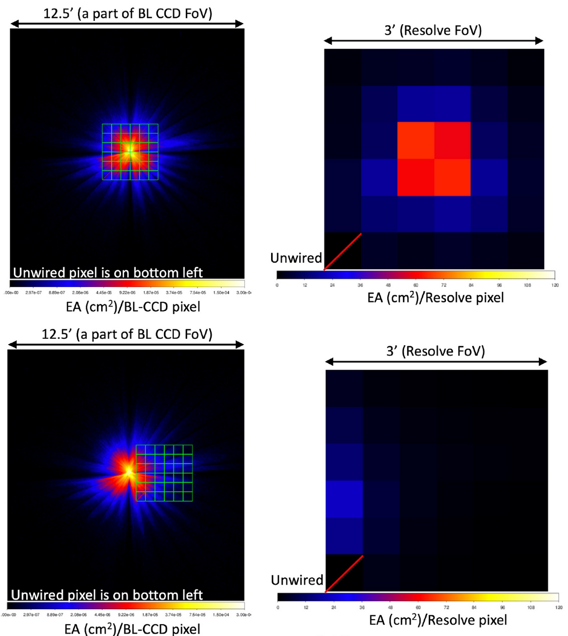
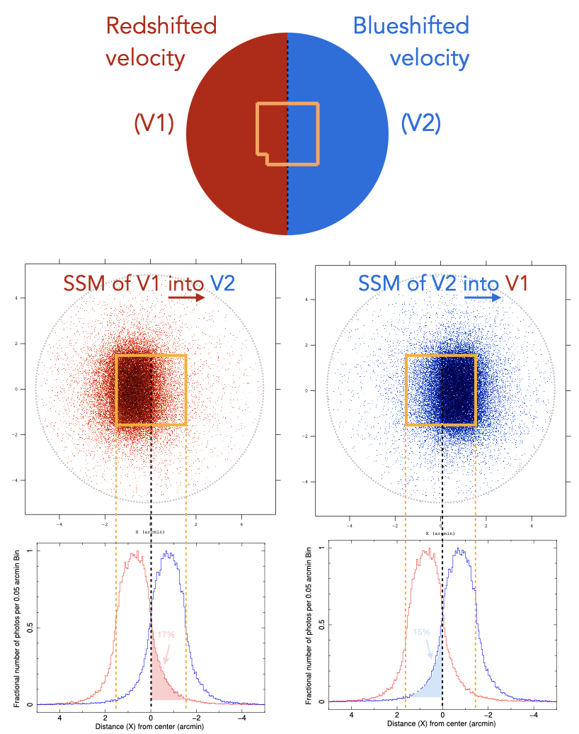
The external and internal SSM are illustrated in Figure 7.1 for the simple case of photons from a single point-like source spreading over the detector. As seen on the figure, due to mirror support structures, imperfect alignments of telescope components, mirror foil figure errors, and non-ideal foil surfaces, the PSF has a complex shape and is not azimuthally symmetric. Particularly in the case of a complex extended structure (e.g., with resolved point sources, clumps and/or hot spots), the PSF effects cannot be seen as a simple Gaussian-like smoothing of an ideal image and should be thus addressed carefully and accurately. The next two figures (Figs. 7.2 and 7.3) focus on a concrete (though very simplistic) case of a circular extended source, half of which is redshifted (V1 = +235 km $s^{-1}$) while the other half is blueshifted (V2 = $-$235 km $s^{-1}$). At first approximation, this is close to what is expected for galaxy clusters with rotating bulk motions of their hot haloes. The spectral effects of the PSF mixing of that specific source are shown in Figure 7.3. Quite interestingly, a mixing of the two components with equal fluxes (e.g., if one looks at central region covering the two components simultaneously) produces a double-peaked line profile, much easier to identify and interpret than the asymmetrical profile seen when one component dominates over the other (e.g., if one looks at a region with one component – though inevitably affected by SSM still).

Generally speaking, the SSM issues described above are somewhat less impactful for Xtend as its PSF (although of similar size as in Resolve) is much smaller than its field of view. Except in specific cases, a moderately extended source placed on axis of the (large) Xtend field of view will thus make the external SSM less important in comparison, and it will be easier to quantify the internal effects of the PSF mixing within the source. Moreover, the moderate spectral resolution of Xtend means that there will inevitably be less subtle spectral features to be affected by SSM. This, however, does not mean that SSM effects can be neglected when analyzing extended sources with Xtend. In fact, variations from e.g., bright emission lines (and/or the continuum) are still important to take into account even at CCD resolution.

The “advantage” of the SSM from Xtend is that the issue is not new. In fact, such effects have affected extended sources in very similar ways in previous missions such as ASCA or Suzaku. For this problem, we thus refer the proposer to the literature which abound with many concrete cases (for the case of galaxy clusters, see e.g., Bulbul et al., 2016; Markevitch et al. , 1996; Bautz et al., 2009). In contrast, the above-mentioned characteristics of Resolve make (internal and external) SSM issues more complicated and relatively unexplored (see however the case of the Perseus cluster observed by Hitomi; e.g., Hitomi Collaboration , 2018). The rest of this chapter will therefore focus primarily on Resolve.

7.2 Facing the challenge: methods and prospects

As mentioned earlier, the problem of SSM is not completely new, as it has already been encountered to some extent in other X-ray missions – in particular those with a large PSF, such as Suzaku and NuSTAR. The spectral analysis of X-ray extended sources in those cases is often performed as follows:

1. Subdivide the extended source in various spatial regions of interest (e.g., where spectral features and physical properties may vary);
2. Extract, for each spatial region, a spectrum ($S_j$) as well as an associated ARF ($A_j$). In most cases, the same RMF ($R_j$) can be assumed for all regions as it weakly varies across the detector;
3. Fit each region with a linear combination of models, where each model $M_i$ is associated with each spectrum $S_j$ as follows:

   $$S_1 = A_{1} R_{1} (P_{1 \rightarrow 1} M_{1} + P_{2 \rightarrow 1} M_{2} + P_{3 \rightarrow 1} M_{3} + …)$$ (7.1)

   $$S_2 = A_{2} R_{2} (P_{1 \rightarrow 2} M_{1} + P_{2 \rightarrow 2} M_{2} + P_{3 \rightarrow 2} M_{3} + …)$$ (7.2)

   $$S_3 = A_{3} R_{3} (P_{1 \rightarrow 3} M_{1} + P_{2 \rightarrow 3} M_{2} + P_{3 \rightarrow 3} M_{3} + …)$$ (7.3)

   $$...$$ (7.4)

   Under a more generic form, one has:

   $$S_j = A_{j} R_{j} (\sum_{i} P_{i \rightarrow j} M_{i}),$$ (7.5)

   where $P_{i \rightarrow j}$ are coefficients corresponding to the relative contribution of the model $M_i$ in the spectrum $S_j$. In an ideal case with no contamination at all, the $P_{i \rightarrow j}$ matrix is in fact diagonal. Even in more realistic cases, many $P_{i \rightarrow j}$ terms may be negligible (particularly if regions $i$ and $j$ are more than a few arcmin away), however the SSM will inevitably make several other $P_{i \rightarrow j}$ values positive.

Figure 7.4: Illustration of the tasks performed by the routine xaarfgen—and the utility of the latter in computing SSM coefficients for the analysis of extended sources.

To estimate numerically each value from the $P_{i \rightarrow j}$ matrix, a tempting approach would be to associate them directly with the normalization parameter of each model $M_i$ in simultaneous fits of all spectra $S_j$. Such normalization parameters ( $N_{i \rightarrow j}$) would then be left free in the fits. This method, however, is strongly discouraged for a number of reasons. First, thawing all these normalizations considerably increases the number of free parameters in the fits, with a high risk of reaching strong degeneracies between the latter and/or local minima in the fits. Also, the best-fit values of the free $N_{i \rightarrow j}$ coefficients may not reflect the true mixing rate in the considered region (as such normalizations could be biased by other unaccounted uncertainties). In fact, free normalizations between the matrix elements uncouple the problem from the actual telescope and detector, making a “black box” of the whole SSM issue, and will thus likely give artificial results. Such approach should be thus avoided by all means, particularly in the case of Resolve observations.

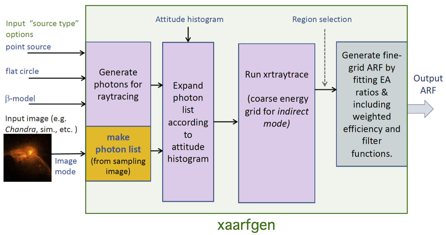
A much more accurate way to proceed is to determine these coefficients directly by calculating (i.e. via ray-tracing) the contribution of each component from region $i$ into a considered region $j$. This can be done from the XRISM data reduction software by the routine xaarfgen (Figure 7.4) which, via its ray-tracing subroutine xraytrace, generates an ARF that can be applied directly on a given model $M_i$. The obtained effective area has been specifically scaled by the routine to account for the exact contribution from region $i$ into region $j$, meaning that the normalization parameter of each model $M_i$ remains untouched (thus, it conserves its initial physical interpretation). The subroutine xraytrace is able generate such ARFs from a geometrically simple input model (e.g., point source, $\beta$ model) or even an input image; e.g,. taken from Chandra/ACIS, XMM-Newton/EPIC, or simply from a simulation^7.1. Adopting this method, the $P_{i \rightarrow j}$ values have their information directly encoded in a grid of ARFs generated specifically for this purpose ( $A_{i \rightarrow j}$), and the above system of equation becomes then:

$$S_1 = R_{1} (A_{1 \rightarrow 1} M_{1} + A_{2 \rightarrow 1} M_{2} + A_{3 \rightarrow 1} M_{3} + …)$$ (7.6)

$$S_2 = R_{2} (A_{1 \rightarrow 2} M_{1} + A_{2 \rightarrow 2} M_{2} + A_{3 \rightarrow 2} M_{3} + …)$$ (7.7)

$$S_3 = R_{3} (A_{1 \rightarrow 3} M_{1} + A_{2 \rightarrow 3} M_{2} + A_{3 \rightarrow 3} M_{3} + …)$$ (7.8)

$$...$$ (7.9)

or, under its generic form,

$$S_j = R_{j} (\sum_{i} A_{i \rightarrow j} M_{i}).$$ (7.10)

In the case of Resolve, it becomes then tempting to follow the same method with, for bright and very extended objects, up to 35 regions (each corresponding to one active pixel on the detector). However, the wealth of spectral information delivered by XRISM associated with the complexity of the ray-tracing process used for the mission requires computing resources that may become considerably heavy. In fact, the computing time requested for ray-tracing in the “fast-mode” (i.e. with more limited off-axis accuracy) and extracting a single ARF can easily exceed the hour, making the above approach extremely time-consuming (i.e. on the order of days or even weeks for standard single machines).

Besides the use of distributed/pseudo parallel computing (if available at the user's host institute), a library of pre-computed PSFs (as a function of the energy, off-axis angle, azimuthal angle) will be made available for Resolve after the launch of the mission (likely ready for AO-2). The sum of contributions will then generate a series of fine-grid effective areas for the spectral regions considered. Another alternative to reduce computing times is to focus on a small energy range^7.2 (if permitted by the science goal) and/or reduce the number of ray-tracing photons. Also, since the SSM is due to the telescope, the ray-tracing code xrtraytrace as part of the XRISM data analysis software can be used to make SSM estimates by running standalone for single energies. For proposals and/or actual analysis of real data, one can still use the above approximate methods to make an initial assessment of which cross-mixing elements are negligible (e.g,. two regions that are distant from each other). Doing so, the run time for creating the full ARFs is not wasted on ARFs that can be safely omitted.

7.3 Consequences and general considerations

As we have seen in the previous two sections, the analysis of extended sources with XRISM is possible, but challenging. To help proposers evaluate to what extent their science goal is feasible, we provide in this section a list of items and considerations that are important to keep in mind at all stages of the observation – from the proposal to the analysis.

We stress that this list is purely indicative, non-exhaustive, and does not constitute a formal checklist for the technical feasibility of any future proposal.

1. It is very likely that the proposers' extended source will be affected by SSM. To estimate how the latter will impact the analysis of the former (and the proposed science goals), it is important to take into account all information on what is known (or unknown) about the spatial and spectral structure of the source. The presence of notable features (e.g., hot spots, blobs, bright nearby AGN or centrally peaked emission), each with their own spectral behavior, will inevitably affect the spectrum of the spatial region(s) to be investigated. Determining how strongly this will affect your science goals and what strategy to use when accounting for this effect will be essential for conducting successful observations.

2. If known to some extent, it is strongly advised to plan a coherent mapping/tiling of the source; i.e. to define spatial regions where pixels are thought to have a (more or less) similar spectral behavior. This also means that, in some cases, the observation should rather be aligned for an optimal match of pixels with spatial features of the source (e.g., to better capture cavities in clusters or shocks in SNRs), rather than simply match the center of the source with the on-axis position of the detector.

3. As the science goal might depend on which region of the extended source (and with which roll angle) the telescope should point at (e.g. if one wants to minimize the SSM in one particular region of interest), it is also important to check the target visibility. This can be done using the visibility checker tool and optimizing the observational position based on the position angle in the observation period.

4. Generating ARFs can be computationally expensive. This is especially true in the case of extended sources, as accounting for the SSM often requires to generate a large number of ARFs. The proposers should keep in mind that several methods exist, some may be more appropriate depending on the proposers' needs and available computing resources (e.g., computing precise ARFs directly, using fastmode, using PSFLib, using an alternative or hybrid method, etc.).

5. A consequence of the previous item is that, although tempting, using Resolve for multi-pixel array spectroscopy is challenging: given that any given pixel is likely affected by the emission from the 34 others, this approach requires the simultaneous fitting of at least 35x35 = 1225 spectral components^7.3. If only one pixel is of particular interest, however, the problem can be considerably simplified by grouping all the others in one common region.

6. The SSM is commonly (and correctly) assumed to happen within the field of view. The external SSM, however, should not be ignored, as its contamination to the investigated sky region(s) can be non-negligible in some cases.

7. Quite counterintuitively, substantial SSM is not necessarily “bad” for the analysis. For instance, a mixing of two components in equal proportions is likely to give rise to spectral features that are easier to spot (and control) than a fainter contamination whose subtle features may lead to significant biases. Specifically, two equally bright regions of different velocities could result in a double-peaked line, much easier to disentangle than a 90-10% mixing resulting in slight (yet significant) line asymmetry.

8. Once the data are retrieved, spectral clues of SSM should rather be investigated by eye before performing a blind fit. Fitting residuals might also provide some clues for mixing (e.g., finding a bump where no line is expected). Similarly, even at the proposal stage it is encouraged to explore the feasibility well beyond a simple setup of fakeit and fitting commands in Xspec.

9. The proposers should keep in mind all other systematic uncertainties that may affect the analysis of their extended source. Effective areas, for instance, have their own uncertainties. Those can be of various origins (e.g., calibration, statistical fluctuations in ray-tracing estimates, or even uncertainties related to software algorithms and assumptions). Similarly, other particular properties of the source might, in some cases, further complicate the analysis (e.g., pileup effects – see Chapter 8, uncertainties in atomic databases impacting spectral features relevant to the science goals, etc.).