|
Next: Spectropolarimetry Example Up: Walks through XSPEC Previous: Producing Plots: Modifying the
Markov Chain Monte Carlo ExampleTo illustrate MCMC methods we will use the same data as the first walkthrough.
XSPEC12> data s54405
...
XSPEC12> model phabs(pow)
...
XSPEC12> renorm
...
XSPEC12> chain type gw
XSPEC12> chain proposal gauss deltas 100.0
XSPEC12> chain walkers 20
XSPEC12> chain length 200000
XSPEC12> parallel walkers 10
We use the Goodman-Weare algorithm with 20 walkers and a total length of 200,000. For the G-W algorithm the actual number of steps are 200,000/20 but we combine the results from all 20 walkers into a single output file. We start the chain with a set of walkers drawn from a multidimensional gaussian whose sigmas are one hundred times the parameter deltas and whose means are the current model parameters. Note that we used the renorm command to make sure that the model and the data have the same normalization. If we had multiple additive parameters with their own norms then a good starting place would be to use the fit 1 command to initially set the normalizations to something sensible.
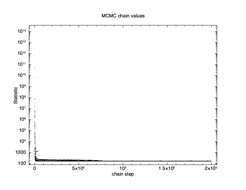
XSPEC12> chain run test1.fits The first thing to check is what happened to the fit statistic during the run. The thin N option on the chain plot means that only every Nth point is plotted. It is important to pick an N which is incommensurate with the number of walkers to make sure that they are sampled equally.
XSPEC12> iplot chain thin 31 0
PLT> log y
PLT> pl
The result is shown in Figure 4.11, which plots the statistic value against the chain step. It is clear that there is an initial burn-in phase before the chain reaches equilibrium so we tell XSPEC to discard the first 100,000 steps and then record the next 200,000.
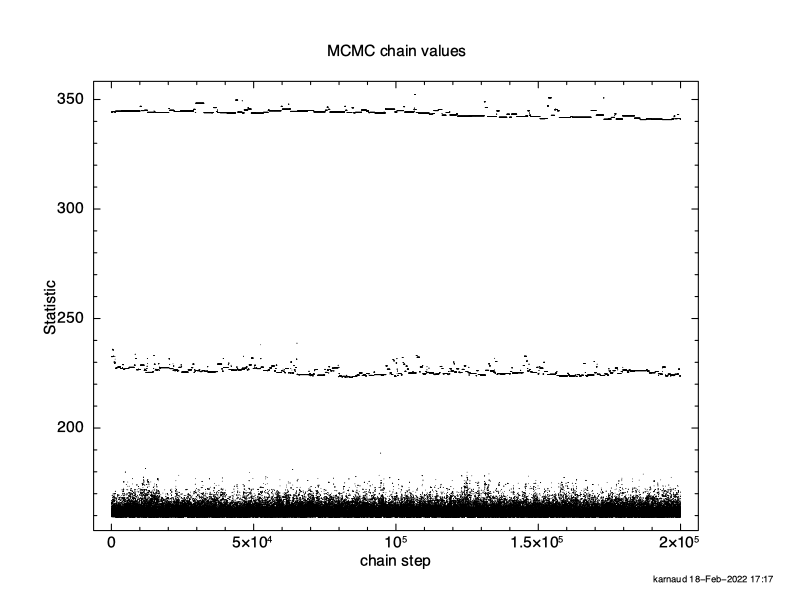
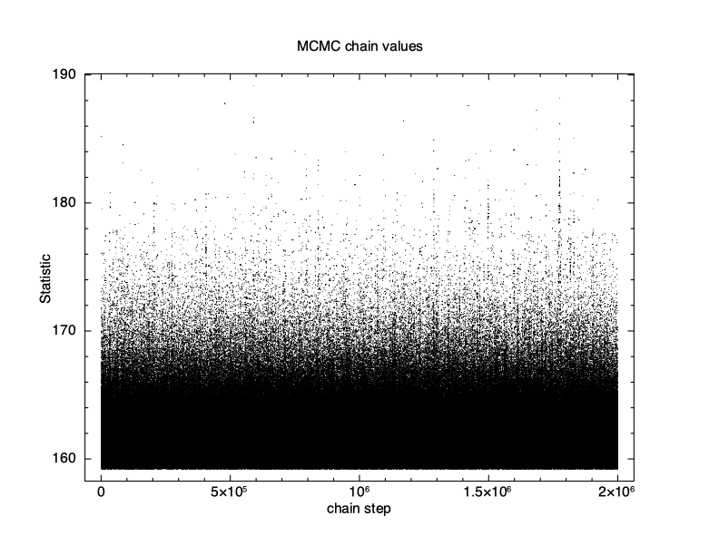
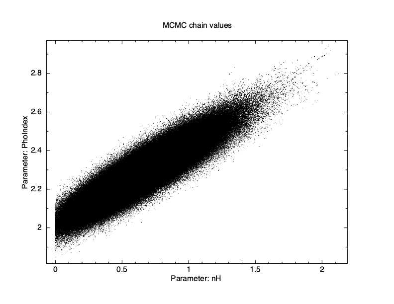
XSPEC12> chain burn 100000
XSPEC12> chain run test1.fits
The result is shown in Figure 4.12, which again plots statistic value against the chain step. What we see is that some of the walkers have not mixed, something which happens sometimes. Finally, we run a chain with ten times as many steps and ten times as long a burn-in to give Figure 4.13. The parameter values can be plotted either singly using e.g. plot chain 2 for the power-law index or in pairs eg plot chain 1 2 giving a scatter plot as shown in Figure 4.14.
Using the error command at this point will generate errors based on the chain values.
XSPEC12>error 1 2 3
Errors calculated from chains

 Parameter   Credible Interval (90\%)
     1     0.202032      1.12274
     2      2.08515      2.49323
     3    0.0102687     0.019415
The 90% confidence ranges are determined by ordering the parameter values in the chain then finding the center 90%.
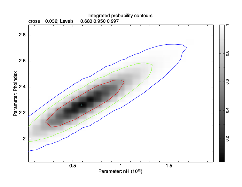
To make confidence regions in two dimensions the margin command takes the same arguments as steppar.
XSPEC12>margin 1 0.0 2.0 25 2 1.8 2.9 25 Then use plot integprob to produce a contour plot of the integrated posterior probability where the contours enclose 68, 95, and 99.7% of the probability (see Figure 4.15).
Next: Spectropolarimetry Example Up: Walks through XSPEC Previous: Producing Plots: Modifying the HEASARC Home | Observatories | Archive | Calibration | Software | Tools | Students/Teachers/Public Last modified: Friday, 23-Aug-2024 13:20:40 EDT |