

Data Simulation and Analysis Threads
Simulate an EPIC or RGS Spectrum with Sherpa
To simulate an EPIC spectrum, we will need an RMF and ARF that correspond to the mode and filter that we are interested in; for RGS, we need only an RMF.
An easy way to get the EPIC RMF and ARF files is to get the responses that are used for PIMMS and WebPIMMS simulations . Alternatively, we could download from the XSA archive an observation that was taken in the mode and filter we want, extract a spectrum and its associated RMF and ARF, and then use those response files to make a simulation. (While the mode and filter information is also in the HEASARC archive, observations are not easily searchable on these.) Note that the ARF is not time-dependent like the RMF is, so one from early in the mission should work well. However, ARFs are dependent on the filter, so be careful to select a dataset with the correct one. Or, if we prefer, we could download an observation in the mode and filter we want and then download a canned redistribution matrix with the corresponding epoch, mode, etc., and generate its corresponding ARF. Canned redistribution matrices for EPIC and RGS can be found through the SOC's calibration portal or the GOF ( PN, MOS, RGS.
We will demonstrate how to simulate a point source, and a source with background.
In this example, we assume that a source spectrum is known to be a power law with photon index=1.9, a Galactic absorption column of NH=5e21 cm-2, and an X-ray flux (0.2-12 keV) = 2.5e-12 erg s-1 cm-2. Let's say that we want to see what exposure time we need in order to measure the hydrogen column density to 2%. We need to initialize CIAO and then call Sherpa. Please note that Sherpa is indentation-sensitive and will throw an error if it detects what it thinks is an indentation when it isn't expecting one.
All of the commands below can be copied-and-pasted into a Sherpa session, as text after the "#" sign is treated as a comment.
   ciao
   sherpa
   set_xsxsect("vern")                      # use the atomic cross sections of Verner et al. 1996
   set_xsabund("wilm")                      # use the elemental abundances of Wilms et al. 2000
   set_source(1,xstbabs.t1 * xspowerlaw.p1) # define the model for the first (and only) source
   t1.nh = 0.5                              # set the model parameters
   p1.phoindex = 1.9
   p1.norm = 1
   fake_pha(1, "m1.arf", "m1.rmf", 2e5)     # make a 200 ks exposure in MOS1 using the named ARF and RMF
   calc_energy_flux(0.2,12)                 # find the flux in erg s-1 cm-2 from 0.2-12 keV; we
                                            # get 4.263640400828176e-09
When we use a normalization = 1, we get an energy flux in this passband of 4.26e-9 erg s-1 cm-2. But we know that the flux for this source should be 2.5e-12 erg s-1 cm-2. This means that we need to scale our normalization accordingly:
( 2.5e-12 erg s-1 cm-2 / 4.26e-9 erg s-1 cm-2) × 1.0 = 0.00058685
Now that we know what the normalization should be, we can continue making our simulation:
   p1.norm = 0.00058685
   fake_pha(1, "m1.arf", "m1.rmf", 2e5)
What if we wanted to simulate a spectrum in RGS? The method is almost exactly the same, the only difference being that RGS does not have an ARF file. So to simulate the R1 and R2 first order spectra, the call to fake_pha would look like this:
   fake_pha(1, None, "R1o1.rmf", 2e5)
   fake_pha(2, None, "R2o1.rmf", 2e5)
Returning our attention to the simulated MOS1 spectrum, we can fit it using the same model that we used when making it, though we should first reset the initial values. We are not grouping the data, so we will use cstat. For the optimization, we'll use simplex (also known as "neldermead"), because it samples the parameter space more thoroughly than the default Levenberg-Marquardt, and is quicker than Monte Carlo ("moncar" in Sherpa parlance).
   ignore(":0.2,12:")                     # ignore data with E < 0.2 keV or E > 12 keV
   set_stat("cstat")
   set_method("simplex")
   t1.nh = 0.1
   p1.PhoIndex = 1.0
   p1.norm = 1e-3
   fit()
   covar()                                # get the uncertainties; this is a simple model, so
                                          # "covar" is sufficient. For complex models, use "conf".
We can see that the fit produced spectrum parameters in excellent agreement with their true values, and the percent error on NH is 2%, so this is a reasonable exposure time for our purposes.
Now we will plot the fit. One thing to keep in mind is that by default, Sherpa does not generate error bars for data points when simulating a spectrum, nor does it read in error bars when loading one (though this can be changed). Instead, it calculates the error bars for each bin using the statistics that are applied during a session. Cstat, however, does not generate error bars -- only flavors of the χ2 statistic do. This means that if we want to compare a fit that was found with cstat to the data and have reasonably accurate error bars, we need to switch to χ2, group the data so it will be Gaussian (or almost Gaussian), and plot the fit on the grouped spectrum.
Also, note that grouping the data should be done after the energy band is defined by the "ignore" (or "notice") command, as used above. This is to avoid having an energy limit accidentally fall in the middle of a bin and that bin getting artificially shortened. This is not likely to have a noticeable effect if a source is bright, but it can if a source is faint.
set_stat("chi2gehrels") # let's use Gehrel's χ2
group_counts(20) # rebin to at least 20 counts per bin
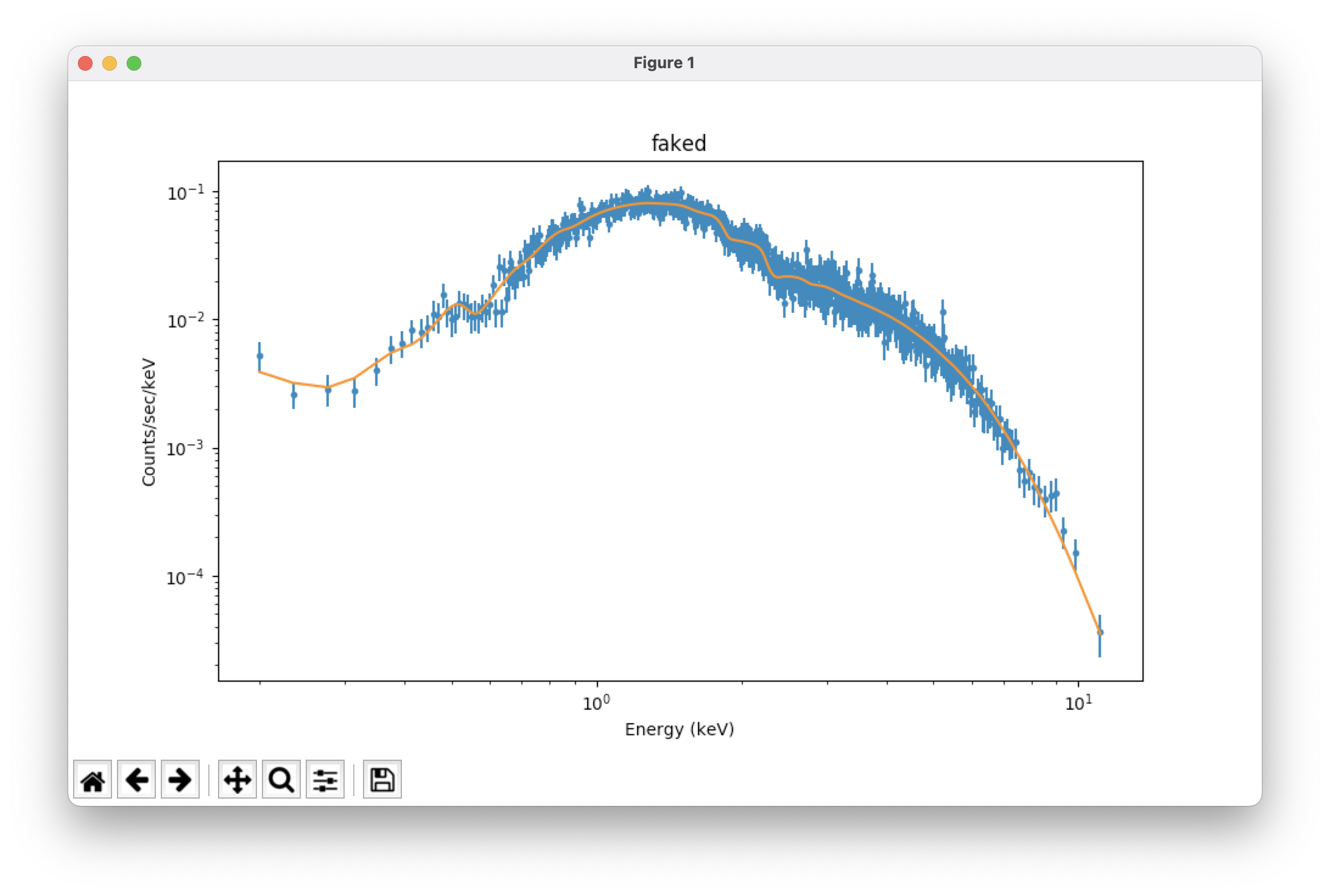
set_xlog() # set the plot axes to the log scale
set_ylog()
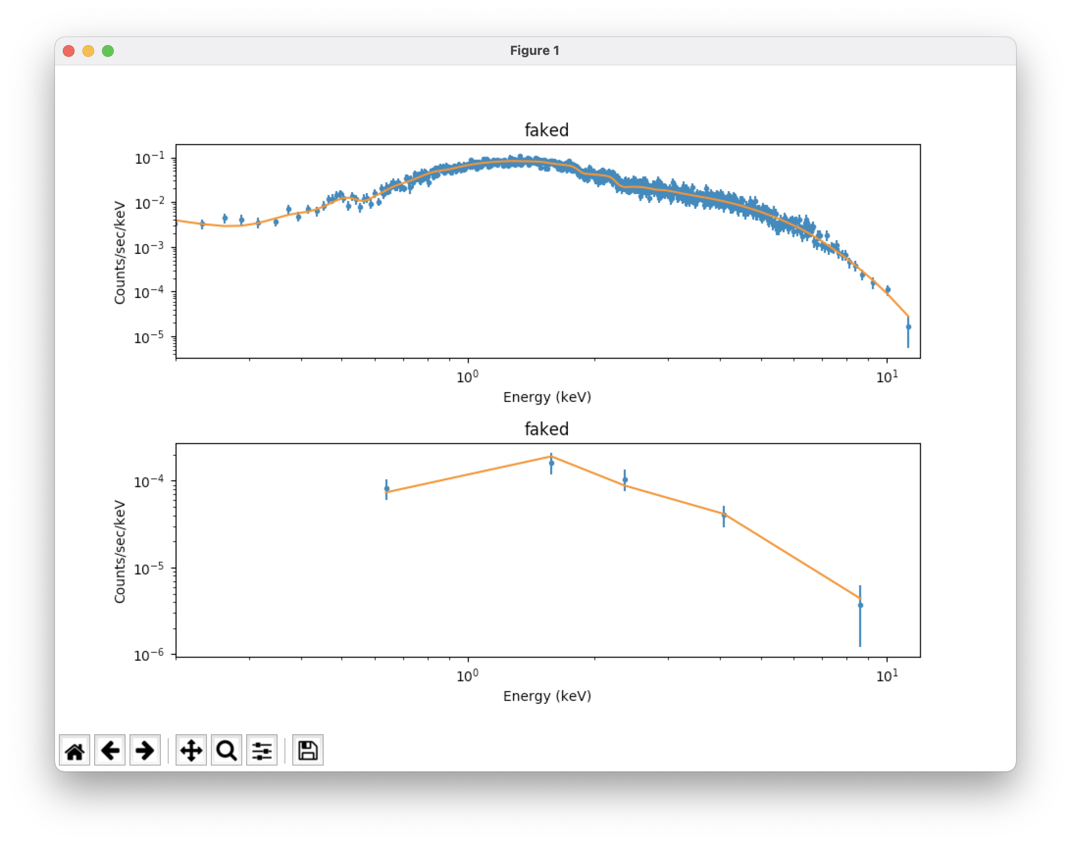
plot_fit() # plot the fit on the data; see Figure 1, top
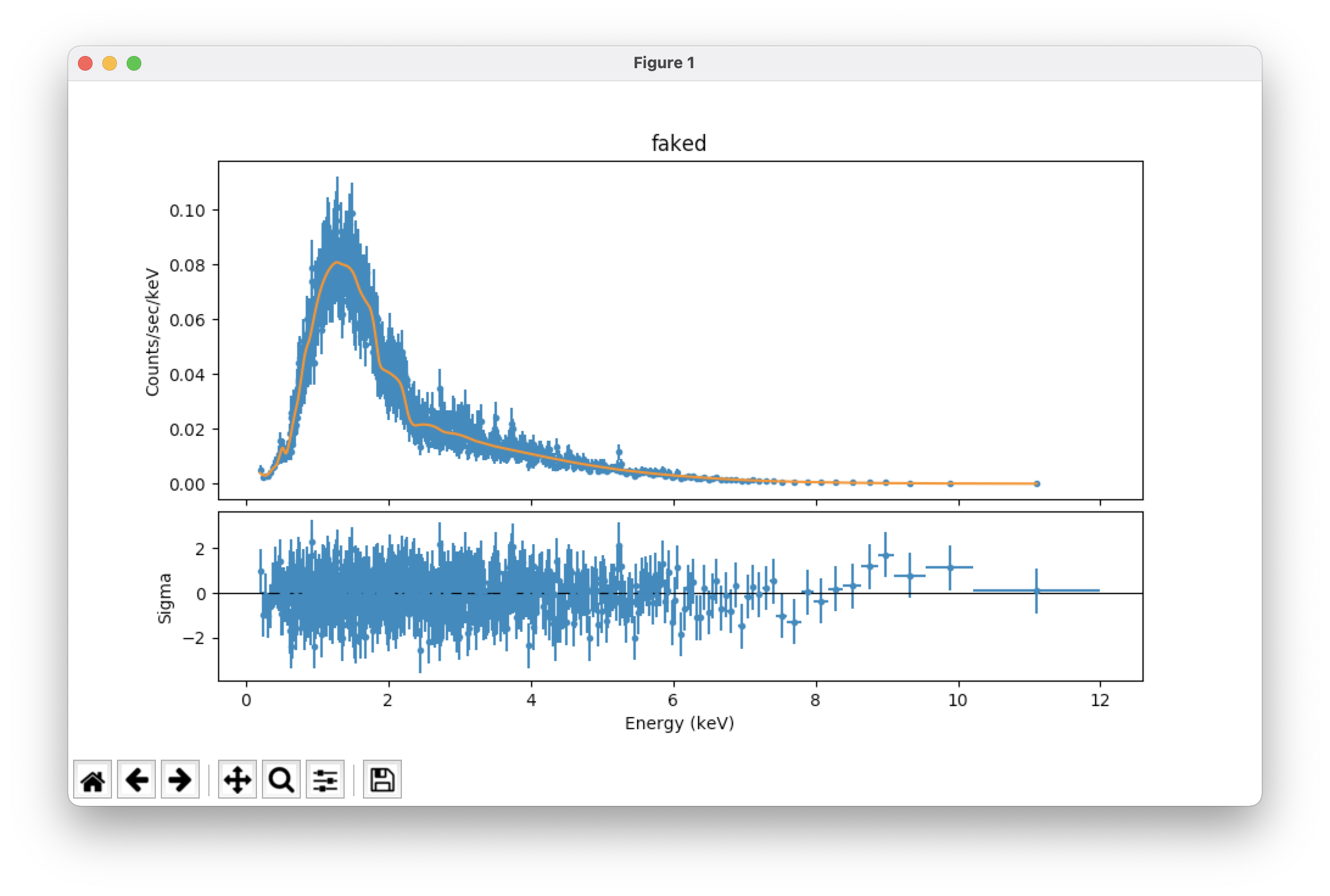
set_xlinear() # set the plot axes to the linear scale
set_ylinear()
plot_fit_delchi() # plot the fit and (data - model)/errors; see Figure 1, bottom
|
|
A Source with a Background Component
We can also simulate a source with a background component. For convenience, we will use the same RMF and ARF as the source, though this isn't necessary. Let's say that it is a standard AGN-dominated background, with photon index = 1.4 and an X-ray flux of about 1e-14 erg s-1 cm-2 in the bandpass. We must first simulate it on its own, to determine its normalization, and we will assume that the interstellar absorption is dominated by material between the source and us (i.e., there is negligible additional absorption in the AGN background).
   clean()                                # erase all data and models in the session and reset the
                                          # choice of statistics and optimization to their defaults
   set_source(xstbabs.t1 * xspowerlaw.p2)
   t1.nh = 0.5
   p2.phoindex = 1.4
   p2.norm = 1
   fake_pha(1, "m1.arf", "m1.rmf", 2e5)
   ignore(":0.2,12:")
   calc_energy_flux(0.2,12)               # flux = 8.786427962152142e-09 erg s-1 cm-2; scaling the
                                          # normalization, we find p2.norm = 1.13812e-06
Now that we have the correct parameters for the background, we can continue generating the spectra.
set_source(1, xstbabs.t1 * xspowerlaw.p1) # set the model for the source
set_source("faked_bkg", xstbabs.t1 * xspowerlaw.p2) # set the model for the background
t1.nh = 0.5
p1.phoindex = 1.9
p1.norm = 0.00058685
p2.phoindex = 1.4
p2.norm = 1.13812e-06
fake_pha(1, "m1.arf", "m1.rmf", 2e5)
fake_pha("faked_bkg", "m1.arf", "m1.rmf", 2e5)
set_bkg(1, get_data("faked_bkg")) # link the background to the source
set_stat("chi2gehrels") # we called "clean", so we already reset the statistic to
# Gehrel's χ2, but there is no harm in doing this again
ignore(":0.2,12:")
group_counts(20) # The background was linked to the source, so it will automatically be
# grouped to the same binning.
set_xlog()
set_ylog()
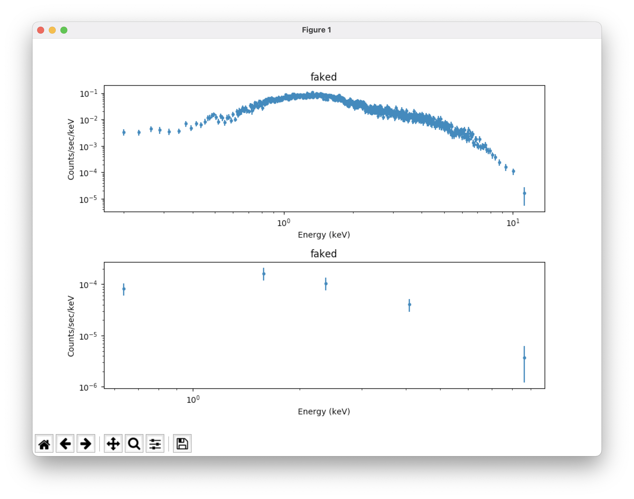
plot("data","bkg") # take a look at our source and background spectra (which
# have appropriate error bars); see Figure 2 (top)
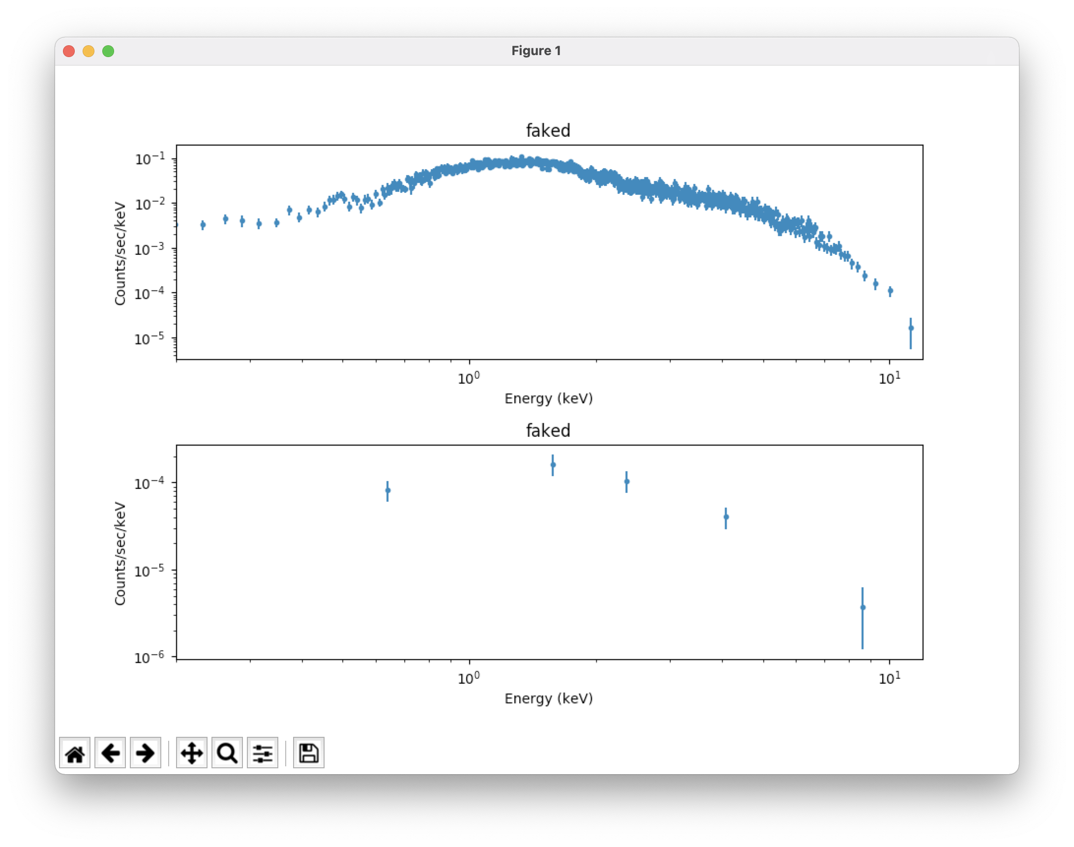
fig=plt.gcf() # set the x axis range for both plots to 0.2-12 keV; see Figure 2 (bottom)
for i in [0,1]:
fig.axes[i].set_xlim(0.2,12)
|
|
Now we'll fit the spectra and plot the result. The background has been linked to the source, but we still need to set the model for it so that Sherpa treats it correctly in the fits. We are not grouping the spectra, so we need to use statistics and optimization that are appropriate.
   ungroup()                              # undo the grouping
   set_stat("cstat")
   set_method("simplex")
   t1.nh = 0.1
   p1.phoindex = 1.0
   p1.norm = 1e-3
   set_bkg_model(xstbabs.t1 * xspowerlaw.p2)  # set the background model
   p2.phoindex = 1.0
   p2.norm = 1e-4
   fit()
   covar()
   calc_energy_flux(0.2,12.)
   calc_energy_flux(0.2,12.,bkg_id=1)     # find the energy flux of the background
   group_counts(20)
   set_stat("chi2gehrels")
   plot("fit","bkgfit")                   # plot the fit to the source and background
   fig=plt.gcf()
   for i in [0,1]:
      fig.axes[i].set_xlim(0.2,12)        # use our chosen energy range in both plots; see Figure 3
|
We can also save our simulated spectra and come back later to fit them.
   ungroup()
   save_pha(1, "mos1_sim_200ks.fits")
   save_pha("faked_bkg", "mos1_sim_bkg_200ks.fits")
   exit()
Note that while Sherpa linked the background spectrum to the source spectrum during the session, it did not write the name of the background spectrum into the BACKFILE keyword of the source spectrum file's header, so we can do that now.
dmhedit mos1_sim_200ks.fits filelist=none operation=add key=BACKFILE value=mos1_sim_bkg_200ks.fits datatype=indef
Now we just load and fit the spectra like any other dataset. The associated response files and background will be loaded automatically:
   sherpa
   load_pha("mos1_sim_200ks.fits")
   ignore(":0.2,12.0:")
   set_stat("cstat")
   set_method("simplex")
   set_xsxsect("vern")
   set_xsabund("wilm")
   set_source(xstbabs.t1 * xspowerlaw.p1)
   set_bkg_model(xstbabs.t1 * xspowerlaw.p2)
   t1.nh = 0.1
   p1.phoindex = 1.0
   p1.norm = 1e-3
   p2.phoindex = 1.0
   p2.norm = 1e-4
   fit()
   covar()
   calc_energy_flux(0.2,12.)
   calc_energy_flux(0.2,12.,bkg_id=1)
   set_stat("chi2gehrels")
   group_counts(20)
   set_xlog()
   set_ylog()
   plot("fit","bkgfit")
   fig=plt.gcf()
   for i in [0,1]:
      fig.axes[i].set_xlim(0.2,12)
   exit()
One final note: it is easy to lose track of things while switching back and forth between types of statistics, optimizations, models, and datasets. The following commands are very useful for assessing where things stand.
   get_stat()      # Print the current statistic and a short description of it to the screen.
   get_method()    # Print the current optimization method to the screen.
   get_xsxsect()   # Print the current atomic cross section setting to the screen.
   get_xsabund()   # Print the current elemental abundance setting to the screen.
   show_model()    # Show all the models that have been defined.
   show_data()     # Show all datasets, RMFs, and ARFs that have been defined.
   show_all()      # Combination of "show_data()" and "show_model()"
If you have any questions concerning XMM-Newton send e-mail to xmmhelp@lists.nasa.gov