Barycenter Correction and Phase Resolved Spectroscopy

Overview

The purpose of this tutorial is to guide users through the process of barycenter correcting their NICER data and then demonstrating how to calculate photon phases from the barycenter corrected arrival times. We will then select certain phases for spectral extraction.

Read this thread if you want to: Barycenter correct your data and perform phase resolved spectroscopy

Last update: 2024-01-30

Introduction

NICER is frequently used to observe sources with an X-ray periodicity (e.g. neutron stars, white dwarfs). It is often desirable to assign a phase to each photon arrival time based on the periodicity of the source, and then to construct a source pulse profile (i.e., phasogram). Once phases are assigned, phase-resolved spectroscopy can also be performed to search for spectral changes as a function of phase. Here we provide a short example of how such an analysis can be accomplished.

In this analysis thread, we will walk through downloading a sample data set, assigning barycentric timestamps, assigning phases, and performing NICER analysis on this data, including phase-resolved spectroscopy.

Prerequisites

To demonstrate this type of analysis we will use an observation of the Crab pulsar. If you would like to follow along with this example, the observation can be downloaded from the HEASARC data archive using the following wget command: wget -q -nH --no-check-certificate --cut-dirs=5 -r -l0 -c -N -np -R 'index*' -erobots=off --retr-symlinks https://heasarc.gsfc.nasa.gov/FTP/nicer/data/obs/2020_03//3013010102/

We use a relatively short observation to keep the data volume small and processing time relatively short.

See How to access NICER data for more information on how to access NICER data.

For barycenter analysis of any target, you will need an accurate celestial position of the target. For microsecond timing accuracy, you will need a celestial position accurate to arcseconds or better.

Specifically, the timing error associated with a position error scales approximately as, Err(t) ~ (2400 msec) * sin(lat) * Err(lat) where lat is the ecliptic latitude, and the error in latitude is expressed in arcseconds. As you can see from this expression, for microsecond-level barycenter absolute timestamp uncertainties, positional uncertainties of the order of milliarcseconds is required, depending on ecliptic latitude, of course. There is an additional timing error term, which is an annual sinusoid, that is due to uncertainty in ecliptic longitude.

This discussion applies primarily to the most sensitive absolute timing accuracy applications, where long term pulsar phase connection is required, over weeks, months and years. For shorter term time baselines (<day), approximate frequency determination, and incoherent power estimation applications, a coarser target position may be tolerable.

For accurate absolute timing analysis with barycentering, a precise celestial position is required.

In our example, we use the Crab celestial position, as reported in the ATNF catalog .

Analysis: Applying Barycenter Correction

First the data should be reprocessed with the nicerl2 task in order to apply the latest filtering criteria and calibrations:

nicerl2 3013010102 clobber=YES

For more discussion of the many options to nicerl2, please see the nicerl2 analysis thread.

Next, we need to barycenter-correct the data. To do this we will use the following command:

barycorr infile=ni3013010102_0mpu7_cl.evt outfile=ni3013010102_0mpu7_cl_barycorr.evt orbitfiles=../../auxil/ni3013010102.orb.gz ra=83.63322 dec=22.014461 barytime=yes

where:

• infile is the name of the input event file
• outfile is the name of the output barycenter-corrected event file
• orbitfiles is the orbit file used to correct the photon arrival times; this is the "orb" file that is found in NICER's aux/ subdirectory.
• ra and dec are the celestial coordinates that will be used to perform the barycenter correction (here they are taken from ATNF).
• barytime is a switch that causes barycorr to add a new column with the ba rycentered times to the output file.

The RA and DEC are optional inputs, if they are not provided barycorr will use the nominal pointing RA and DEC of NICER. This is usually the desireable behavior, but if NICER has been offset-point, or if the target position in the input files is incorrect or inaccurate, this will lead to inaccurate barycenter results. For this reason, and for the reasons of documenting results for publication, users should always double-check the celestial coordinates of the target. If barytime is set to NO, (which is the default value) the original times in the output file will be overwritten with the barycenter corrected times. See below for a more in-depth discussion of the the barytime YES/NO question.

barytime=YES or barytime=NO?

Most tutorials for barycentering X-ray data recommend setting barytime=NO. Here we are recommending to set barytime=YES, and we describe why in this section.

When barytime=NO, the barycorr tool will overwrite the existing TIME column with barycentered timestamps. The old TIME values are lost. Depending on the target declination and season of the year, the new barycentered timestamp values will have a difference of up to ~500 seconds from the original non-barycentered timestamp values.

Downstream NICER software does not work properly with barycentered timestamps in the TIME column. Other auxiliary files such as the filter files and FPM selection information are NOT barycentered. As noted above, there is up to a 500 second difference in timestamp values. When calculating response matrices and background estimates, which use these auxiliary files for interpolation by time, this time offset leads to incorrect estimates of response and background.

One approach might be to apply barycenter correction to all files, including the filter file and FPM selection information, etc. However there are some technical difficulties with this approach that are to detailed to describe here, and we cannot recommend this approach.

When you set barytime=YES, barycorr keeps the original TIME column intact and unchanged, and it writes a new column called BARYTIME. The BARYTIME column has the new barycentered timestamp values. We will use this to our advantage with NICER software.

NICER software will automatically use the TIME column for temporal filtering, background estimation, and response generation. Since the TIME column is unchanged when you set barytime=YES, the NICER tools will report accurate results. All of the new information is encoded in the BARYTIME column, which we can used to encode pulse phase information, as described further below.

There are some disadvantages to using barytime=YES. The main one is that some downstream timing software packages rely upon barycentered timestamps being reported in the TIME (not BARYTIME) column. Also some metadata keywords such as TIMESYS are not modified when barytime=YES, and this may confuse some downstream software as well.

Thus, our recommendation is to run barycorr with barytime=YES for NICER spectral and light curve analysis, including pulse phase spectroscopy as described below. If you plan on feeding barycentered NICER data to downstream tools, you should run barycorr again, with barytime=NO and a separate output file, and use that file only for the downstream tools (but not NICER products).

Analysis: Applying Phases

Once the data have been barycenter corrected, we need to assign phases. In order to do this an ephemeris is needed. The ephemeris can either be provided from external sources (e.g., the Crab is frequently monitored by Jodrell Bank Observatory and their ephemeris can be found here: https://www.jb.man.ac.uk/pulsar/crab/crab2.txt ) or from your own timing analysis if a periodicity is found in the data.

Prior to calculating the phases, it may be easiest to create a new time column with the reference time (epoch) of the ephemeris subtracted from the barycenter corrected times. Alternatively, this can be folded into the phase calculation. The ephemeris reference for the crab data is MJD 58917 plus 0.025552 seconds. Using the HEASARC xtime tool, we can convert this MJD time to the NICER mission elapsed time of 195177602.000 seconds.

To subtract this reference time from the barycenter corrected time, we use the command: ftcalc infile='ni3013010102_0mpu7_cl_barycorr.evt[events]' outfile=ni3013010102_0mpu7_cl_barycorr.evt column=BARY_REF_TIME expression='(BARYTIME-(195177602.000+0.025552))' clobber=yes where:

• infile and outfile are the names of the input file and output file. Here we are overwriting the baryceter corrected file in place, which is why clobber=YES is needed. Also note that the events extension is selected, so ftcalc knows in which extension to place the new column, which is why we need quotation marks.
• column is the new column name, which we call BARY_REF_TIME.
• expression is mathematical expression that ftcalc will calculate and place into the new column, which subtracts the epoch reference time as described above.

Phases can then be assigned using an ftcalc command like this: ftcalc infile='ni3013010102_0mpu7_cl_barycorr.evt[events]' outfile=ni3013010102_0mpu7_cl_barycorr_PHASE.evt column=PHASE expression='(29.6095750017*(BARY_REF_TIME)+(-368174.57e-15*(BARY_REF_TIME**2)/2))%1' where:

• infile is the event file with subtracted epoch reference time
• outfile is the new file with PHASE column added
• column is the new phase column, called PHASE
• expression is the mathetmatical expression to calculate phase

The expression here calculates phase as phase = f * T + 0.5 * fdot * T^2 where f and fdot are the frequency (29.6095750017 Hz) and frequency derivative (-368174.57e-15 Hz/s), as determined by your pulsar timing analysis. T is the epoch time, which is BARY_REF_TIME in this case. The frequency and frequency derivative are from the Crab ephemeris.

The "%" symbol is the CFITSIO calculator modulo operator. In this case, "modulo 1" means to take the fractional part of the value, after removing the whole number portion. Thus, we obtain the fractional phase, from 0.0 - 1.0.

The approach described here computes PHASE using an a priori known frequency and frequency derivative, and results in a fractional spin frequency between 0 and 1.

Once we have our phases, we can open and plot the phasogram using fv. This can be done using the command:

fv ni3013010102_0mpu7_cl_barycorr_PHASE.evt

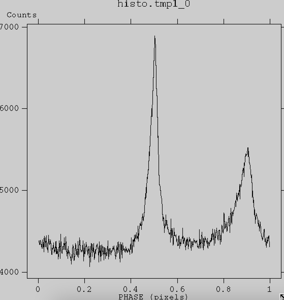
With the event file open, you can click "HIST", then select "PHASE" for the x-axis. Next click "Make" and you should see the following plot.

Figure 1. Phasogram of the Crab pulsar produced by the above commands and plotted using fv.

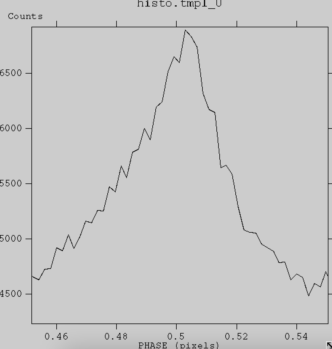
Here we can see the pulse profile of the Crab pulsar as observed by NICER. We can zoom in on the first pulse peak by clicking and dragging our cursor to form a box surrounding this segment. This will zoom in on the peak and it should look like the image shown below.

Figure 2. Phasogram zoomed in on the first pulse peak from the Crab pulsar produced by the above commands and plotted using fv.

Analysis: Phase-Resolved Spectroscopy

In order to extract the spectrum of just the first X-ray peak, we need to select the start and stop phases of the peak. Since this is simply a demonstration, we select by eye the phases 0.45-0.55 to cover the first peak. In practice, the analyst will chose phase ranges that suit the particular source and pulse profile.

Now that we have determined the start and stop phases, we are ready to create a custom Good Time Interval (GTI) file. To accomplish this task, we will use the maketime ftool, which can be used to create custom GTI files. The input to maketime is the event file containing the calculated phases and the output file directory/name. Then we add a statement to filter on the start and stop phases of the first puslar peak. The ".and." selects the times between the phases.

The expression looks like this: maketime infile=ni3013010102_0mpu7_cl_barycorr_PHASE.evt outfile=3013010102/xti/event_cl/peak_gti.fits expr="((PHASE >=0.45).and.(PHASE <=0.55))" NAME VALUE time=TIME compact=no clobber=yes where:

• infile is the event file with PHASE column
• outfile is the new GTI file
• expr is the phase selection expression, which in this case selects fractional phases 0.45-0.55
• NAME, VALUE and compact=NO are dummy arguments which are relics from a time when maketime worked with "compact" housekeeping files (which NICER does not use)
• time=TIME indicates to report GTIs using the TIME (not BARYTIME) column.

Here, the (barycentered) PHASE column is used for selection of GTIs, but the (unbarycentered) TIME column is used to construct the GTI start and stop times. Thus, the GTIs are not barycentered and can be used to filter unbarycentered NICER event files, but the selection is based upon properly barycentered pulsar phases.

Once we have made the GTI file, we can perform a few checks to make sure the file was created correctly. The first check is to simply open the file with fv, click "All" in the STDGTI extension and make sure there are GTIs in the file.

Another, more rigorous check, is to check that the correct phases were selected by repeating the steps outlined above. To accomplish this, we first move the folder we were working in to a different name. Next, we rerun nicerl2 with the new GTI file as follows:

nicerl2 3013010102 gtifiles=3013010102/xti/event_cl_full/peak_gti.fits clobber=yes

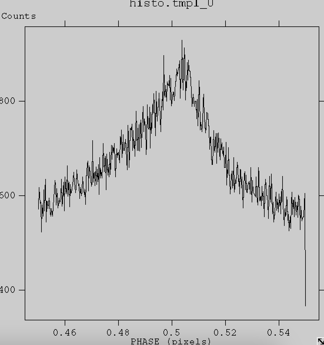
Once this is done, the phases can be recalculated by repeating the steps outlined above. You can then plot them again using fv to ensure that the correct phases were selected. You should see an image similar to Figure 3.

Figure 3. Phasogram of the Crab pulse peak produced by the above commands and plotted using fv. Note the histogram will look different due to fv choosing a large number of bins. The bin size can be changed by changing the "Bin size" value when plotting.

If you performed this check and verified the result, then you can simply run nicerl3-lc on the newly produced files that were created by running nicerl2 with the new GTI file in the standard way (i.e., you do not need to provide a GTI file to nicerl3).

Since we are using an event file which has an unbarycentered TIME column, the nicer spectral response and background estimates will be correct.

Alternatively, if you are confident that the phase selection worked properly and do not want to rerun everything again, the phase resolved spectrum can simply be extracted using (however see the caveats for the 3C50 model):

nicerl3-spect 3013010102 suffix=peak gtifile=3013010102/xti/event_cl/peak_gti.fits clobber=YES

where:

• 3013010102 is the observation directory
• gtifile is the gti file we made using maketime
• suffix is a special suffix, so we can distinguish this spectrum from others

Analysis: Correcting EXPOSURE for Partial Phase Coverage

When using maketime to create GTIs, the exposure will only be approximately correctly calculated for sufficiently bright sources, such as the Crab pulsar. However, if you are working with a fainter source, it is safest to update the exposure keyword in the header file of the spectrum. The correct exposure time can be calculated by multiplying the total exposure time by the size of the phase been used.

For example, this observation has a total exposure time of 224 seconds, and we selected a phase bin of size 0.55-0.45=0.1. Therefore, the correct exposure time should be 0.1*224=22.4 s. This exposure time can be manually added to the header of the extracted spectrum using the following command:

fthedit 'ni3013010102mpu7_srpeak.pha[1]' keyword=exposure operation=add value=22.4 unit=s comment='updated exposure time' where:

• ni3013010102mpu7_srpeak.pha[1] is the name and extension number of the file in which the header will be edited. We use quotation marks because of the '[1]' extension number
• keyword is the keyword to be edited, exposure in this case
• operation is 'add' to add or modify the EXPOSURE keyword
• value is the value to change the exposure to and unit is the value's units
• Comment is the description of the updated exposure time

The NICER team recommends to adjust the exposure for spectra obtained with this approach, because the phase selection results in reduced effective livetime.

Now the spectrum can be loaded into xspec and fit using the standard procedures. The correct exposure time will be automatically read into xspec.

Caveats

Note that the 3C50 background model is currently not supported when using nicerl3-spect with a GTI file. A workaround to this is to run nicerl2 with the custom GTI file (shown above as a check on the GTI file), and then run nicerl3-spect on that output from nicerl2. In this case no GTI file needs to be passed to nicerl3-spect.

No Orbit File?

In some cases you may not have an orbit file. This may be because you have quicklook data products or only access to a subset of NICER data. It is still possible to perform barycentering, but with reduced accuracy.

Given NICER's trajectory in low earth orbit, a typical maximum error incurred by not using an orbit file is about 40 light-milliseconds. For many objects, including slow pulsars or systems with timing noise, accuracy better than 40 msec may not be required. In that case, you may not need an orbit file to perform barycentering.

You may not need an orbit file, if you can tolerate 40 msec timing uncertainty errors in the resulting barycentered timestamps. This will be specific to your source and timing application.

If that is the case, you can run barycorr as follows, barycorr ... orbitfiles=GEOCENTER ... where orbitfiles=GEOCENTER indicates a detailed orbit file is not required. The "..." indicate that all other parameters to barycorr can be entered unchanged as described further above.

Modifications

• 2023-11-30 - initial draft