Recognizing and Dealing with Non-X-Ray Flares in NICER Data

Overview

This page discusses "flares" that may be seen in NICER data. It deals with possible mitigation approaches to removing them.

Read this thread if you want to: Recognize and Deal with Flares in NICER Data

Last update: 2024-02-14

Introduction

The NICER observatory is designed to point at and record X-rays from an astrophysical target, such as a star, neutron star, or AGN. X-rays enter the NICER aperture, are concentrated by the X-ray Concentrator optics and detected by a Focal Plane Module, where they are recorded and transmitted to the ground for analysis.

Unfortunately, in addition to X-rays, the NICER detector system is sensitive to other things besides X-rays. These "other" things are also recorded and transmitted to the ground and are also potentially visible in NICER event data.

The source of non-X-ray events can be:

• non-X-ray background
• noise events
• undershoots and overshoots (internal NICER detector behaviors)

For a broad discussion of types of NICER backgrounds, please see the SCORPEON overview page.

Non-X-ray events are a nuisance, and we desire ways to remove, account for, or screen out such events. Here, we will focus on non-X-ray background events, and in particular, "flare-like" episodes.

For a non-imaging detector like NICER, non-X-ray flares are a significant nuisance, because there is no way to use imaging data or off-source data to determine if a flare is "real" or not. This page discusses techniques used to recognize and deal with flares in NICER data.

Please be aware that this is a topic of ongoing analysis and research. Some of these techniques are not 100% reliable, and may serve more as indicators than iron-clad guarantees of flaring or clean data. Human judgement is required.

Types of Flares

Here we summarize the types of non-X-ray flares that might be seen in NICER data.

Precipitating Electron Flares. This is perhaps the most frequent kind of flare observed in NICER data. According to the discussion on the SCORPEON overview page, precipitating electron events are caused by magnetic reconnection events that occur in the outer magnetosphere, which channel electrons along magnetic field lines to the north and south polar horn regions. The flares caused by these events can be particularly intense, but also very faint. They typically last from seconds to minutes.

Low-Energy Electron Flares. These rarer events are less well understood but appear to be correlated with solar substorm events. The spectrum tends to be softer than precipitating electron flares, and the duration is in the hours to days time frame. Such events are more often seen in the equatorial regions.

Noise Flares. In rare circumstances, extremely high optical loading causes the NICER noise peak to become very intense and broadened. These effects are strong enough to cause the noise peak to extend into the nominal X-ray band. We will now discuss these types of flares in more detail.

Precipitating Electron Flares

Electron precipitation events occur when trapped electrons in the outer magnetosphere are disturbed. This can occur when a magnetic reconnection event happens, or if other geomagnetic events perturb the electrons. In that case these normally trapped electrons can become untrapped and move down into the lower magnetosphere where NICER is located.
Figure 1. Representation of electrons precipitating from the plasma sheet onto the polar horn regions.

Precipitating electrons are represented by the "prel" component of the SCORPEON model.

General Properties of Precipitating Electron Flares

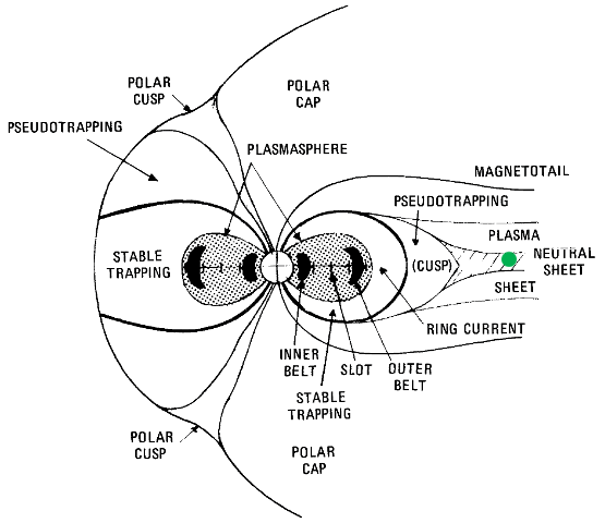
Where. NICER detects these events almost entirely in the polar horn regions. These geographic regions are depicted in the following geographic map.
Figure 2. Map of NICER overshoots as a function of geographic longitude and latitude. The regions where precipitating electrons can be prominent are highlighted in red.

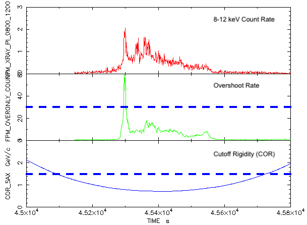
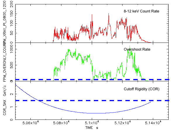
Precipitating electron events are primarily in the north and south polar horn regions identified in the figure.

These regions can be described using the filter file column COR_SAX < 1.5. Here COR_SAX is a representation of charged particle penetration ability, and the polar horn regions are especially penetrable.

When. Electron precipitation events are not particularly predictable.

Intensity. Electron precipitation events can be as intense as 70,000 ct/s for the full NICER array, and as faint as a few counts per second.

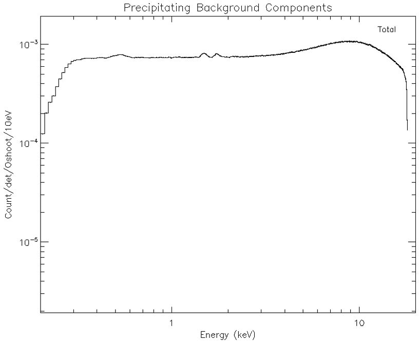
Spectrum. The spectrum of precipitation events, as observed by NICER is often very flat, with a small hump around 8 keV or higher, followed by a rolloff at high energies. Small fluorescence lines at 1.4 and 1.8 keV may be visible in the brightest flares. The following figure shows the average of many such flares taken from NICER background data.
Figure 3. Example spectrum of NICER precipitation events.

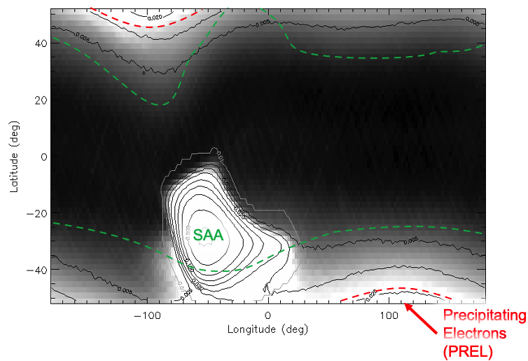
Variability. Precipitation events can be highly variable and structured. You may find a single peak, many small peaks, or rapidly evolving intensity.

Recognizing Precipitation Flares

Recognizing precipitation flares in NICER data is not always easy, but there are some common identifying features.

Precipitation flares are almost always limited to COR_SAX < 1.5 COR_SAX represents regions where charged particles can penetrate closer to the earth, where smaller means larger penetration. We use the COR_SAX filter file column to indicate this ("COR" meaning "cutoff rigidity" and "SAX" meaning "BeppoSAX", whose software is used to compute this filter file value).

Overshoots are often elevated. The overshoot rate during precipitation events is often elevated compared to the times before and after the event. Overshoot rates for the strongest flare events can be as high as ~1000 ct/s/FPM. The standard overshoot screening range of 0-30 reomves these. However, precipitating electron flares can be of all possible intensities, even very faint.

Techniques to Diagnose Flare Candidates

This section describes is a technique to examine an individual flare and assess whether it is astrophysical or not.

We will be using the fplot command to plot three columns from the filter file. We are using fplot here because it is available to anyone that has HEASoft, but you are free to use any software you wish that can plot FITS tables, including "fv".

The input to fplot will be the filter file. Every observation has a filter file, and by default this file is located in NNNNNNNNNN/auxil/niNNNNNNNNNN.mkf where NNNNNNNNNN is the observation ID number. The file may also be gzipped (i.e. have a ".gz" suffix).

Here we will use a background data set, observation 1034100110, which we downloaded from the archive and ran nicerl2 on. The resulting filter file is located in 1034100110/auxil/ni1034100110.mkf.gz.

We will run fplot 1034100110/auxil/ni1034100110.mkf.gz offset=YES where offset=YES is optional but makes displaying numbers on the X-axis a bit more readable.

If you are using "fv" you would run fv 1034100110/auxil/ni1034100110.mkf.gz

We will choose the following plot options:

• X-axis: TIME
• Y-axis: FPM_XRAY_PI_0800_1200 FPM_OVERONLY_COUNT COR_SAX
• List of rows:"-" (fplot only)
• Device:"/xs" or "/xw" (fplot only)
• Any legal PLT command" " (blank space; fplot only)

A plot of the entire range will appear. In the fplot PLT interface, you can use the "r x" command to choose X-axis range, and then combinations of "win 2" "win 3" and "win 4" and "r y" to set the y range for each window. For more information on PLT commands, you can see the QDP/PLT User's Guide.

If you use fv instead, you can use the mouse to choose X and Y ranges for each plot.

Why are we choosing these columns to plot?

• FPM_XRAY_PI_0800_1200 is the count rate for pulse heights in the nominal 8-12 keV band. For many sources there are few counts in this band but the precipitating electron spectrum peaks in this band. In the filter file the column name has the word "XRAY" but these counts can include non-X-rays as well.
  NOTE: if your X-ray target has a lot of counts in the 8-12 keV band, you should be careful you are not seeing variability from the target.
• FPM_OVERONLY_COUNT is the count rate of "overflow" pulses, or pulse heights that exceed about 20 keV. These are typically non-X-ray particle counts instead of X-rays. For more information see the Overshoot Introduction page.
• COR_SAX is the cutoff ridigity, or COR, for NICER as it passes through the earth's magnetic field. High particle backgrounds are often seen at low COR. COR is measured in units of GeV/c.

Together, these quantities can help diagnose the nature of flare-like features seen in NICER data.

Here are two example ranges in the data set we are examining.

Figure 4. Observation 1034100110 plots of 8-12 keV rate, overshoots, and cutoff ridigity (COR) from top to bottom, for an earlier time. The nominal overshoot range of 0-30 ct/s for standard nicerl2 processing is shown in the middle panel; a COR value of 1.5 is highlighted in the bottom panel.

Figure 5. Observation 1034100110 plots of 8-12 keV rate, overshoots, and cutoff ridigity (COR) from top to bottom, for a later time. The nominal overshoot range of 0-30 ct/s for standard nicerl2 processing is shown in the middle panel; a COR value of 1.5 is highlighted in the bottom panel.

Figure 6. Example of a flare caused by precipitating electrons in the 0.5-10 keV light curve of DS Tuc with 35 s bins. Note these flares occur when COR_SAX is below 1.5 (black horizontal line) and also cause an increase in the FPM_OVERONLY_COUNT rate (image credit M. G. Dethero).

Both of these figures show non-X-ray flares of the electron precipitation type, although they are of very different magnitude. The first figure shows data from earlier in the data set, where the COR dips below 1.5 GeV/c.

There are several important things to see here.

Electron precipitation flares almost always occur when COR_SAX falls below 1.5 GeV/c. There are of course always rare exceptions to the rule, but genenerally speaking, precipitation events are governed by the earth's magnetic field, and are therefore channeled to the polar horn regions where COR_SAX is lowest.

Flares are usually highly variable. You may see spiky behavior, or more trending-type variability. Precipitation events are governed by the population of electrons in the outer magnetosphere, the disturbance that perturbs them (which itself can be highly variable), and the magnetic fields that channel electrons earthward. These properties often lead to highly variable behavior.

The overall amplitude can be quite variable. As you can see, the difference in amplitude between the two plots is more than one order of magnitude, despite the data being taken only ~1 orbit apart from each other. In fact, flares of one order of magnitude larger and smaller have been seen, compared to what has been displayed, so flares are particularly pernicious.

The default range of overshoots when processing with nicerl2 or nimaketime is 0-30, which is shown on the plots above. It can be seen that many flaring occassions can be removed with this cut, but others are not. That means that some flares can remain even after the default screening.

In-band counts are not strictly correlated with overshoots. Although overshoots are a good measure to indicate when particle background levels are high, there is not a one-to-one correlation between in-band ("X-ray") count rates and overshoot count rates. This is likely due to the fact that the electron spectrum itself varies in shape, meaning that for each overshoot count (>20 keV), there are a variable number of electrons registered in the <20 keV band. However, overall overshoot variability and trends are a good indicator of high flaring activity.

The spectrum is flat and does not correspond to an X-ray spectrum. The NICER detector system is comprised of XRC gold optics as well as FPM detectors. Each of these introduces characteristic signatures in the spectrum which are not apparent in electron flares. The reason is simple: NICER thermal films, optics and detector windows all introduce X-ray edges into the effective area curve. X-rays and X-rays alone are modulated by these atomic edge effects; electrons are not. Thus, we can use these edges as diagnostics to distinguish between electron flares and X-rays.

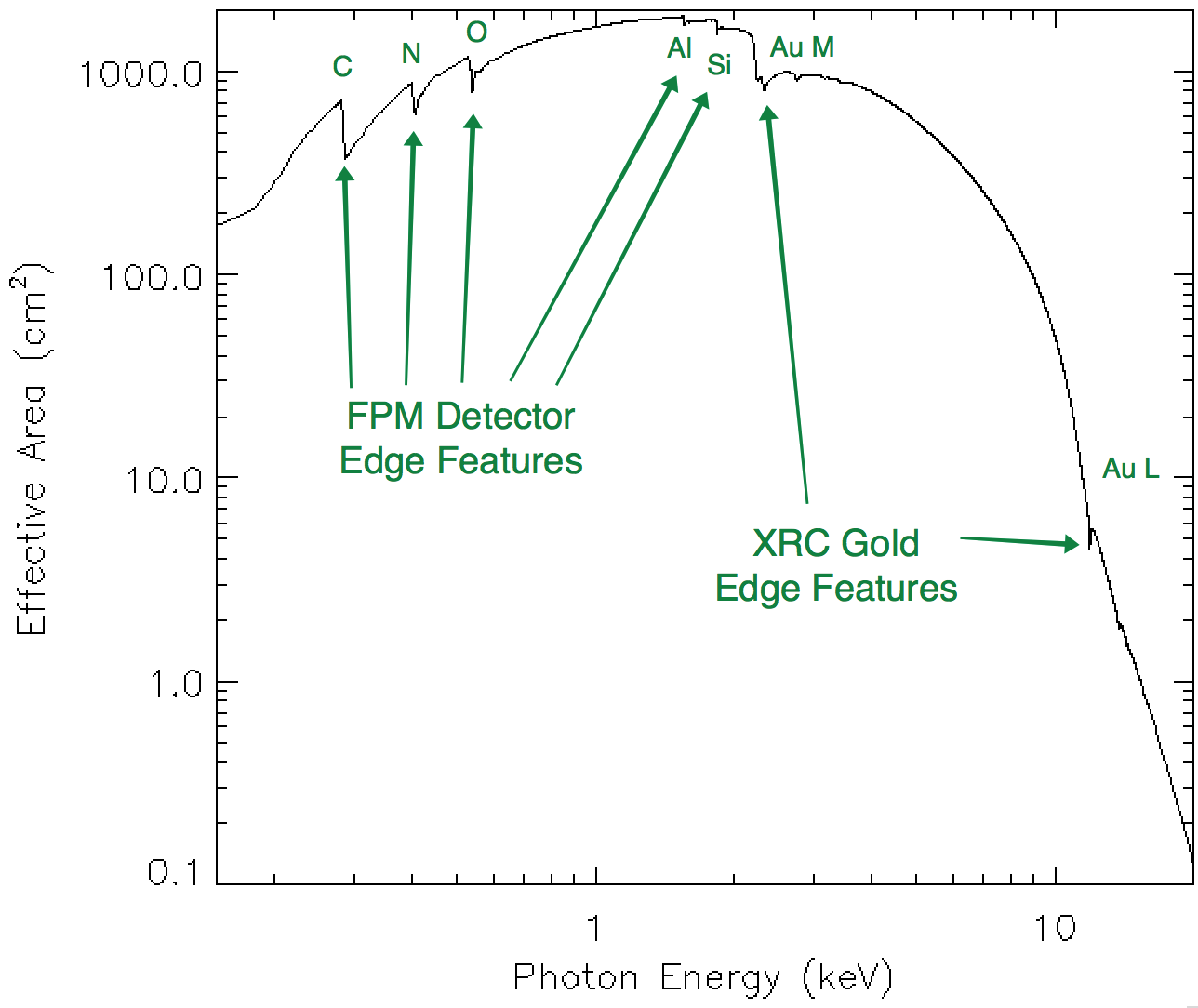
To show this, here we reproduce the figure in the NICER Responses page.
Figure 7. NICER full-array ARF (sum of 52 operating modules). Key detector and optics features are identified.

Every X-ray that passes through the NICER optical system will be affected by the displayed curve. The strong features that are apparent in the effective area curve are:

• Gold M edge near 2.2 keV
• Gold L edge near 10.5-13 keV

Electron flares will NOT have these features because they are not due to X-rays. As shown in Figure 3 above, the typical spectrum of electron precipitation flares is very flat and featureless around 2.2 keV. This is the signature feature that will be in real X-ray spectra that are not in electron spectra.

Using the niprelflarecalc Tool to Diagnose Flares

As of HEASoft 6.33, the NICER team has released a tool called niprelflarecalc. This tool is specially designed to find PREL-related flares.

The NICER team does not recommend nipreflarecalc for automated usage. Rather we are seeking feedback for how the tool works for different scientific applications from the user community.

The niprelflarecalc tool is designed to look at two diagnostic values: the overshoot rate and the "ratio-rejected" counts, sometimes known as "HREJ" counts. Ratio-rejected counts are due to high energy particles that deposit their energy deeply within the silicon detector. PREL flares, by contrast, are dominated by low energy electrons that are not able to penetrate deeply into the silicon. By noting the difference between overshoots and ratio-rejected counts, it may be possible to distinguish moderate to bright PREL flares.

The niprelflarecalc tool can be used to produce additional columns, similar to those that would appear in the standard filter file. In essence, you only need your filter file, and niprelflarecalc will append the new columns.

Run niprelflarecalc like this: niprelflarecalc NNNNNNNNNN/auxil/niNNNNNNNNNN.mkf INFILE clobber=YES where NNNNNNNNNN/auxil/niNNNNNNNNNN.mkf is the location of your filter file and NNNNNNNNNN is your 10-digit observation ID number. If you keep your filter file elsewhere you can adjust the path accordingly. The "INFILE" tells the task to modify the filter file in-place. If you want to make a new copy, you can specify a new file name explicitly.

After you run niprelflarecalc, you will find two new columns in the output file.

• PREL_FLARE_INDEX - a numerical "flaring index" which is intended to indicate times of higher PREL flares. The units are arbitrary, although the index is intended to indicate significance in number of sigma.
• PREL_FLARE_EST - an estimate of the flaring intensity, in arbitrary units.

The NICER team's preliminary recommendation is that the threshold for PREL flares is (PREL_FLARE_INDEX > 4.5), i.e. greater than 4.5 sigma. This criteria will select most weak flares. For strong flares, there may be tails or wings of PREL-related counts that extend beyond the 4.5 sigma threshold.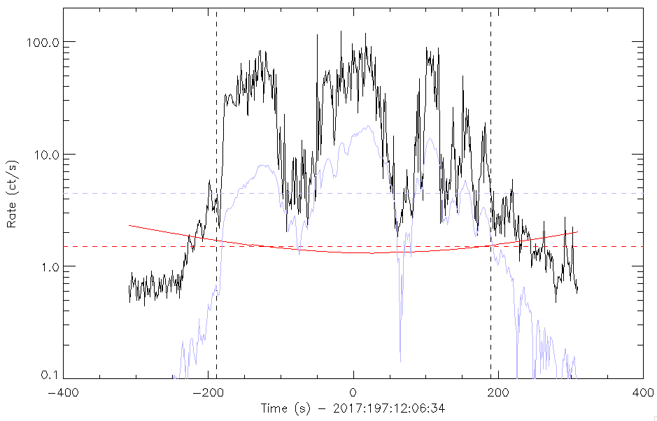

Figure 8. Example of results from running niprelflarecalc. The X-axis is time, and the Y-axis is both count rate and cutoff rigidity in units of GeV/c. Overshoots (black) and cutoff-rigidity (COR, red) are shown, along with the recommended COR_SAX screening threshold of 1.5 (red dashed). The light blue line shows the PREL_FLARE_INDEX, and the light blue dashed line shows the recommended threshold cut of 4.5

Figure 8 shows the results of running niprelflarecalc on a particular data set. The light blue trace shows the estimated PREL_FLARE_INDEX value, which becomes strong especially during passages through polar horn regions (where COR_SAX < 1.5). When the index exceeds a value of 4.5 (sigma), a PREL flaring episode is extremely likely.

Another tool, niprelflaregti, can be used for GTI screening data based on the flaring index. Run this tool like this, niprelflaregti niNNNNNNNNNN.mkf nonflare.gti where niNNNNNNNNN.mkf is the path to your filter file and nonflare.gti is the resulting GTI which should be (mostly) flare-free.

This GTI can be used in combination with nicerl2 or nicerl3-spect to extract spectra with flares removed. Run nicerl2 with the "gtifiles" parameter: nicerl2 ... gtifiles=nonflare.gti and nicerl3-spect ... gtifile=nonflare.gti

niprelflaregti has some safeguards to avoid "shredded GTI" problems, It also combines and extends flaring sections even if the flaring index is just below the threshold. This helps remove tail or wing emission that is part of the PREL flare but below the formal 4.5 threshold. The principle here is that PREL flares are bad and it is better to exclude more data around a flare than less. Once an intense PREL flare is found with a somewhat conservative threshold, the task is more liberal at excluding data with marginal PREL index values.

Mitigating or Handling the Effects of Electron Precipitation Flares

There are a number of approaches that can be used to accomodate the presence of these types of flares. Here we will focus upon spectral analysis.

• Spectral modeling of the flares as background component
• Screening or exclusion of flares

Which avenue you choose depends on what type of science you are after and how bright your X-ray target is expected to be.

Faint and Bursting Targets

If your target is expected to be faint, or you are interested in burst-like behavior from your X-ray target, and the burst-like behavior is of scientific interest, the best solution is to exclude as much potentially bad data as possible.

The benefit of this approach is that you will likely exclude most of the electron precipitation like flares. The downside of this approach is that this kind of conservative filtering may throw out some good data. In the case of faint or burst-like sources, this is probably a good trade-off. The goal is to remove as many non-X-ray flares as possible to reduce the chances of false detection of an X-ray burst.

You can apply these same approaches for intermediate and very bright targets as well, but benefits may be diminishing.

Specific recommendations for dealing with this type of target are:

• Exclude COR 0-1.5 GeV/c range by setting the cor_range=1.5-* parameter when running nicerl2.
• Reduce the allowed overshoot range to 0-5 ct/s instead of the default 0-30, with the overonly_range=0-5. You can try reducing the range even smaller, but may run into problems of "shredded" GTIs or more good data being excluded. Please note that the "normal" range of overshoots for quiescent data is about 0-1, so a range smaller than that will be harmful.
• Examine the spectrum of any flare-like features and determine by eye whether they have the 2.2 keV edge feature or not. You can also try modeling the precipitating electron background as noted in the next section.

If you follow these suggestions, your nicerl2 command will change from nicerl2 NNNNNNNNNN .... clobber=yes to nicerl2 NNNNNNNNNN overonly_range=0-5 cor_range="1.5-*" ... clobber=YES where NNNNNNNNNN is the observation ID. Here you need to put quotation marks around the "1.5-*" portion in order to avoid the Unix shell's wildcard expansion. The "..." represents any other options that you are also using when running nicerl2.

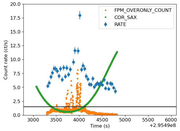
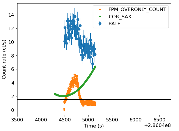
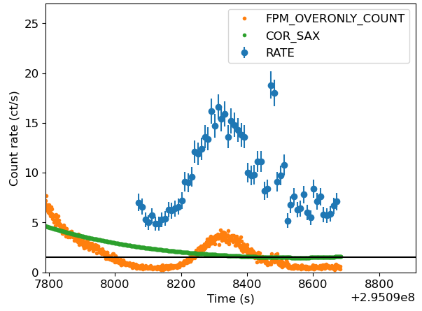
As a side note, if you are experimenting with various screening levels and re-running nicerl2 multiple times, you do not have to wait for nicerl2 to completely re-process everything from the raw data. You can use the "tasks" and "incremental" parameters of nicerl2 to avoid lengthy reprocessing. Please see the Making nicerl2 Run Faster section of the nicerl2 page.

When publishing papers, it is worth describing what screening you have done in your manuscript, such as default or non-default settings so that other researchers can reproduce your results.

Intermediate or Bright Targets

For intermediate or bright targets, you may wish to try other strategies. The strategies listed above the "Faint" section may also be used, of course. However, keeping slightly flaring data and modeling it may be more effective than excluding it. The NICER team still recommends to remove very intense flares, which the default overonly_range=0-30 setting should accomplish.

For these types of targets, it is possible to model the effects of electron precipitation events with background modeling. The three available NICER background models treat precipitation flares differently and you will get different quality results from each.

This approach is to basically use the default settings during screening and spectral extraction, and take no explicit steps to remove or reduce flares. Instead, you model the spectral contribution using a spectral background model.

Please note that this form of modeling explicitly handles the 2.2 keV edge features noted above. Any flares will be attributed to background, which do not use the same ARF as the X-ray source.

The SCORPEON model is specifically designed to handle electron precipitation events. The XSPEC model form of SCORPEON's output has a term called "prel_norm", which is the normalization of the precipitating electron (or "prel") component. By default, SCORPEN will set prel_norm to be unfrozen in XSPEC if COR_SAX dips below 1.5 GeV/c, which is the zone where such flares are most likely to be found. At any time you can also manually unfreeze this parameter. It is strongly advised to fit the spectrum with prel_norm variable if you suspect you have an electron precipitation event.

The 3C50 model has some capability to distinguish between different types of backgrounds and will attempt to adjust its output to match conditions. However, users should be aware that 3C50 does not have a strong ability to distinguish between electron precipitation flares and other types of background. Since precipitation flares can be highly variable, the 3C50 model may not be able to pick up on the nuances of a particular flare.

The Space Weather model is not particularly designed to handle precipitation events. Its training variables are the geomagnetic activity index Kp, which varies slowly over hours to days, and COR_SAX, which varies with geography only. It will not be able to distinguish been a normal pass through the polar horns and a pass through the polar horns with a large flare.

Correlated Variability

Even with the more strict filters outlined above, some flares can still make their way into the data. In the two figures below we show examples of background flares that occur when COR_SAX (green points) is >1.5 and FPM_OVERONLY_COUNT is mostly below 5 cts/s. These flares can be manually screened out by looking for correlated variability in the FPM_OVERONLY_COUNT (orange points) and source count rate (blue points).

Figure 9. Example of a background flare occuring when COR_SAX is > 1.5 and FPM_OVERONLY_COUNT is relatively low (~<5 cts/s). These types of flares can cause correlated variability in the 0.3-7 keV source light curve (blue points; 10 s bins).

Figure 10. Another example of a background flare causing correlated variability in the 0.3-7 keV source light cuve (images produced by M. G. Dethero).

Understanding and Mitigating Low Energy Electron Flares

This section will be published at a later date.

Modifications

• 2023-07-11 - initial draft; precipitation flares only
• 2024-02-14 - updated to discuss niprelflarecalc and niprelflaregti