Extracting a Spectrum During a Flare/Burst

Overview

This tutorial is designed for users who have a burst or flare in their dataset and wish to extract a spectrum corresponding to that feature in the light curve. If you have already identified the flare, it is useful to have the start and stop times determined in NICER mission time, but these times can also be obtained using NICER light curves as demonstrated below.

Read this thread if you want to: Extract a spectrum from a flare or bust

Last update: 2023-07-19

Introduction

NICER often observes highly variable X-ray sources, which may show flaring or bursting behavior. It is often useful to break the observation into several pieces to understand how the source's spectrum evolves with time. Here we provide a short example of how such an analysis can be accomplished.

To demonstrate this type of analysis we will use an observation of the source Swift J1858.6-0814, which is an accreting NS LMXB that showed a type I X-ray burst. If you would like to follow along, the observation can be downloaded from the HEASARC data archive using the following wget command: wget -q -nH --no-check-certificate --cut-dirs=5 -r -l0 -c -N -np -R 'index*' -erobots=off --retr-symlinks https://heasarc.gsfc.nasa.gov/FTP/nicer/data/obs/2020_03//3200400122/

See How to access NICER data for more information on how to access NICER data.

Analysis

First the data should be reprocessed with the nicerl2 task in order to apply the latest filtering criteria and calibrations: nicerl2 3200400122 clobber=YES

Next, a light curve needs to be made so that we can select the times of the X-ray burst which we will use to extract the spectrum from. We will make a 5 s binned light curve in the 0.5-10 keV energy range using the following command: nicerl3-lc 3200400122 50-1000 5 suffix=0.5_10keV_5s clobber=YES where:

• 3200400122 is the observation directory
• 50-1000 is the channel range, here 0.5-10 keV
• 5 is the the time bin size in seconds
• suffix is a special suffix, so we can distinguish this 0.5-10 keV light curve from others

The above parameters (e.g., energy, bin size) can be adjusted to match the needs of your science.

Once we have our light curve, we can open and plot it using fv. This can be done using the command: fv 3200400122/xti/event_cl/ni3200400122mpu7_sr0.5_10keV_5s.lc

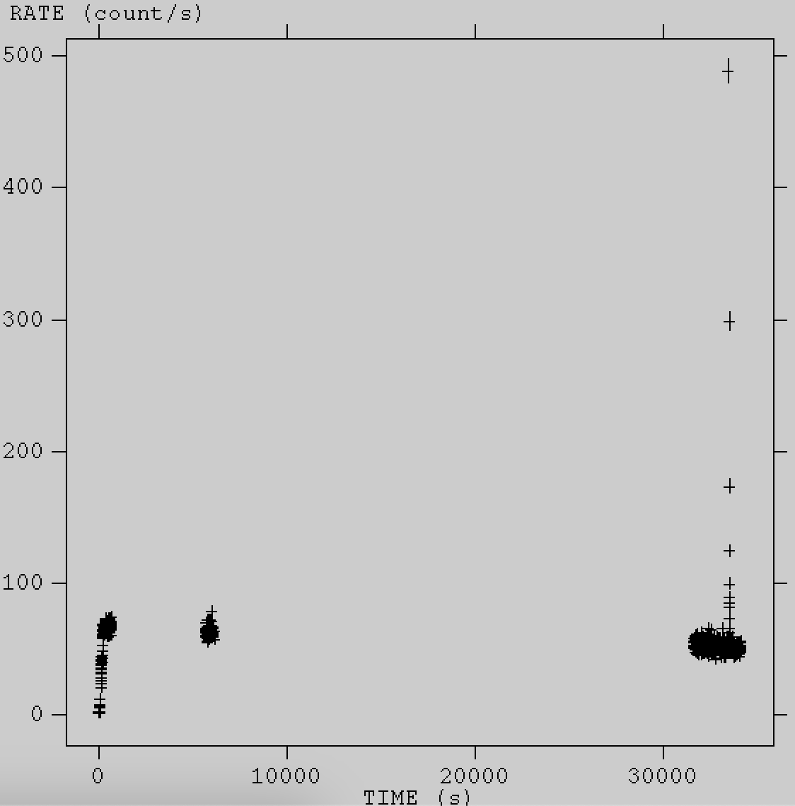
With the light curve file open, you can click "Plot", then select "Time" for the x-axis, "RATE" for the y-axis, and "ERROR" for the "Y Error". This will produce the following plot.

Figure 1. Light curve of Swift J1858 produced by the above commands and plotted using fv.

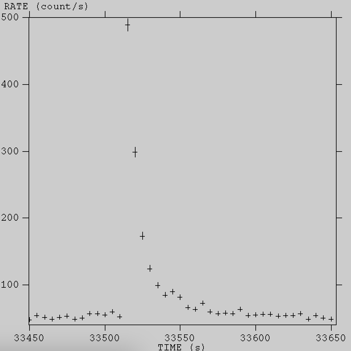
There is a very bright burst seen in the third segment of the observation. We can zoom in on this segment by clicking and dragging our cursor to form a box surrounding this segment. This will zoom in on the segment. From there we can further zoom in on the burst by repeating this procedure and it should look like the image shown below.

Figure 2. Light curve zoomed in on the type I x-ray burst from Swift J1858 produced by the above commands and plotted using fv.

In order to extract the spectrum of just the X-ray burst, we need to use the start and stop time of the burst. However, these times must be given in mission time but the light curves are not given in this time system. Therefore, we need to convert the light curve times to the corresponding mission times. To do this, we can use the following command: fkeyprint 3200400122/xti/event_cl/ni3200400122mpu7_sr0.5_10keV_5s.lc[1] TIMEZERO exact=yes

This command searches for and prints the TIMEZERO keyword from the light curve extension. This is needed because it provides the start time of the light curve in mission time. Running this command should print "TIMEZERO= 1.963268645000000E+08 / Time Zero". So this is the time we will use to convert to the mission time. Now we will extract the times of burst from the light curve. Since this is a demonstration, we will not be very strict on extracting the spectrum at the exact start of the burst, we will simply use a 100 s interval from 33500 to 33600, which captures the burst (see Figure 2). More precise filtering can be done by using a finer time binning to make the light curve, and then plotting it using, for example python, to extract more accurate start and stop times.

Now that we have the start and stop times of the burst, as well as the conversion to mission time, we are ready to create a custom Good Time Interval (GTI) file. To accomplish this task, we will use the maketime ftool, which can be used to create custom GTI files. The input to maketime is the input mkf file and the output file directory/name. Then we add a statement to filter on the start and stop time of the flare. These times are obtained by simply adding TIMEZERO to the light curve times (33500 and 33600) as such: TSTART=196326864.5+33500=196360364.5, TSTOP=196326864.5+33600=196360464.5 The ".and." selects the times between TSTART and TSTOP. maketime 3200400122/auxil/ni3200400122.mkf 3200400122/xti/event_cl/flare_gti.fits "((TIME >=196360364.5).and.(TIME <=196360464.5))" anything anything TIME no clobber=yes

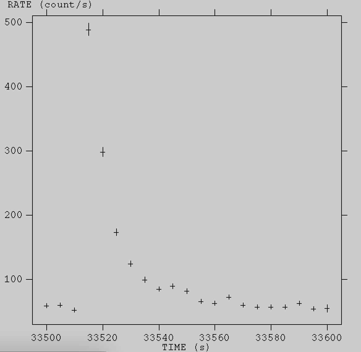
Once we have made the GTI file, we can perform a few checks to make sure the file was created correctly. The first check is to simply open the file with fv, click "All" in the STDGTI extension and make sure the start and stop times agree with those given to maketime. Another quick check that can be performed is to remake the light curve supplying the newly created GTI file using (note the changed suffix!): nicerl3-lc 3200400122 50-1000 5 suffix=0.5_10keV_flare_5s gtifile=3200400122/xti/event_cl/flare_gti.fits clobber=YES

When the light curve is plotted in fv it should look like this figure.

Figure 3. Light curve of the type I x-ray burst from Swift J1858 produced using our GTI files and plotted using fv.

Now that we have confirmed that our GTI file is producing the expected behavior, we are ready to extract our spectrum. The spectrum can be extracted by supplying the GTI file to nicerl3-spect as follows:

nicerl3-spect 3200400122 suffix=flare gtifile=3200400122/xti/event_cl/flare_gti.fits clobber=YES where:

• 3200400122 is the observation directory
• gtifile is the gti file we made using maketime
• suffix is a special suffix, so we can distinguish this spectrum from others

Once the spectrum is produced, we can again double check that the appropriate GTI was applied by loading the data into XSPEC using the load file and checking that the exposure time is 100 s.

Caveats

Note that the 3C50 background model is currently not supported when using nicerl3-spect with a GTI file. A workaround to this is to run nicerl2 with the custom GTI file, and then run nicerl3-spect on that output from nicerl2. In this case no GTI file needs to be passed to nicerl3-spect.

Here we did not apply any barycenter correction to the photon arrival times. This should be done if more accurate time filtering is required.

In some NICER datasets, it may be unclear if the flare/burst you are seeing is real or not. Please see our page on How to determine whether a flare is from the source or background for more information on this topic.

Modifications

• 2023-07-19 - initial draft