

THE XMM-NEWTON ABC GUIDE, STREAMLINED
EPIC-PN (TIMING mode), SAS GUI
Contents
Prepare the Data
Reprocess the Data
Introduction to xmmselect
Apply Standard Filters
Make a Light Curve
Extract the Source and Background Spectra
Check for Pile Up
My Observation is Piled Up! Now What?
Determine the Spectrum Extraction Areas
Create the Photon Redistribution Matrix (RMF) and Ancillary File (ARF)
Prepare the Data
Please note that the two tasks in this section (cifbuild and odfingest) must be run in the ODF directory. These are the only tasks with that requirement, and after this section, we will work exclusively in our reprocessing directory.Many SAS tasks require calibration information from the Calibration Access Layer (CAL). Relevant files are accessed from the set of Current Calibration File (CCF) data using a CCF Index File (CIF).
To make the ccf.cif file, first make sure the environment variables are set:
   cd ODF
   setenv SAS_ODF /full/path/to/ODF/directory/
   setenv SAS_ODFPATH /full/path/to/ODF/directory/
Next, call cifbuild from the SAS GUI. A window with the parameter options will appear; the defaults should be fine, so just click "Run".
To use the updated CIF file in further processing, you will need to reset the environment variable SAS_CCF:
setenv SAS_CCF /full/path/to/ODF/ccf.cifThe task odfingest extends the Observation Data File (ODF) summary file with data extracted from the instrument housekeeping data files and the calibration database. It is only necessary to run it once on any dataset, and will cause problems if it is run a second time. If for some reason odfingest must be rerun, you must first delete the earlier file it produced. This file largely follows the standard XMM naming convention, but has SUM.SAS appended to it. After running odfingest, you will need to reset the environment variable SAS_ODF to its output file. To run odfingest and reset environment variable, call odfingest from the SAS GUI. As before, a pop-up window with the parameter options will appear; the defaults should be fine, so just click "Run". (It is safe to ignore the warnings.)
To change the environmental variable, type
setenv SAS_ODF /full/path/to/ODF/full_name_of_*SUM.SASYou will likely find it useful to alias these environment variable resets in your login shell (.cshrc, .bashrc, etc.).
Reprocess the Data
To reprocess the data, make a new working directory and from it, call epproc or epchain.cd .. mkdir PROC cd PROCThen, close and re-open the SAS GUI, so that it will place the output files in the new directory, and call your preferred pipeline task. Epproc will automatically detect the science mode of the data, so just click "Run". (It is safe to ignore the warnings.) However, epchain does not, so in the "General" tab, toggle the datamode parameter to TIMING and click "Run".
By default, the tasks do not keep any intermediate files they generate. Epproc designates its output event files with "TimingEvts.ds", and epchain follows the standard naming convention. In any case, it is convenient to rename the event file something easy to type:
mv 1192_0400550201_EPN_S003_TimingEvts.ds pn.fitsor
mv P0400550201PNS003TIEVLI0000.FIT pn.fits
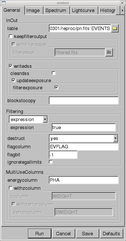
Introduction to xmmselect
The task xmmselect is used for many procedures in the GUI. Like all tasks, it can easily be invoked by starting to type the name and pressing enter when it is highlighted.When xmmselect is invoked a dialog box will first appear requesting a file name. You can either use the browser button or just type the file name in the entry area, "pn.fits:EVENTS" in this case. To use the browser, select the file folder icon; this will bring up a second window for the file selection. Choose the desired event file, then the "EVENTS" extension in the right-hand column, and click "OK". The directory window will then disappear and you can click "Run" on the selection window.
When the file name has been submitted the xmmselect GUI will appear, along with a dialog box offering to display the selection expression; this is shown in Figure 1. The selection expression will include the filtering done to this point on the event file, which for the pipeline processing includes for the most part CCD and GTI selections.
Different event files can be loaded into xmmselect by going to "File -> New Table".

Apply Standard Filters
The filtering expression for the PN in TIMING mode is:
(PATTERN <= 4)&&(PI in [200:15000])&&#XMMEA_EP
The first two expressions will select good events with PATTERN in the 0 to 4 range. The PATTERN value is similar the GRADE selection for ASCA data, and is related to the number and pattern of the CCD pixels triggered for a given event. Single pixel events have PATTERN == 0, while double pixel events have PATTERN in [1:4].
The second keyword in the expressions, PI, selects the preferred pulse height of the event. For the PN, this should be between 200 and 15000 eV. This should clean up the image significantly with most of the rest of the obvious contamination due to low pulse height events. Setting the lower PI channel limit somewhat higher (e.g., to 300 or 400 eV) will eliminate much of the rest.
Finally, the #XMMEA_EP filter provides a canned screening set of FLAG values for the event. (The FLAG value provides a bit encoding of various event conditions, e.g., near hot pixels or outside of the field of view.) Setting FLAG == 0 in the selection expression provides the most conservative screening criteria and should always be used when serious spectral analysis is to be done on PN data.
To filter the data using xmmselect,
- Enter the filtering criteria in the "Selection Expression" area at the top of the xmmselect window:
(PATTERN <= 4)&&(PI in [200:15000])&&#XMMEA_EP
- Click on the "Filtered Table" box at the lower left of the xmmselect GUI. This will bring up the evselect GUI.
- In the "General" tab, change the filteredset parameter, the output file name, to something useful, e.g., pn_filt.fits.
- Click "Run".
Make a Light Curve
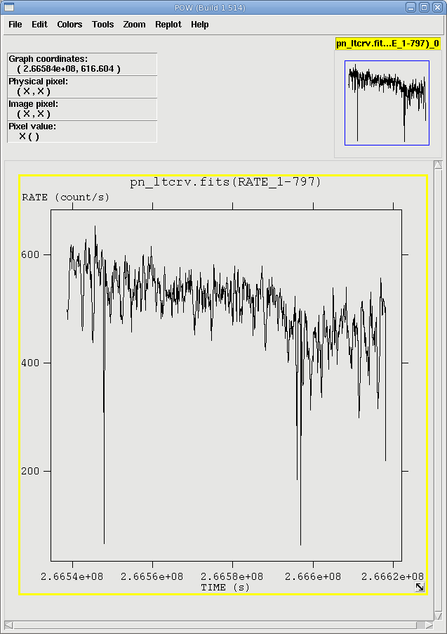
Sometimes, it is necessary to use filters on time in addition to those mentioned above. This is because of soft proton background flaring, which can have count rates of 100 counts/sec or higher across the entire bandpass. To determine if our observation is affected by background flaring, we can make a light curve by calling xmmselect and loading the event file as shown above. Then,
- Check the round box to the left of the "Time" entry.
- Click on the "OGIP Rate Curve" button near the bottom of the page. This brings up the evselect GUI (see Figure 2).
- Click on the "Lightcurve" tab and change the "timebinsize" to a reasonable amount, e.g. 50 s. In the "rateset" textbox, enter the name of the output file, for example, pn_ltcrv.fits.
- Click on the "Run" button at the lower left corner of the evselect GUI.
The output file pn_ltcrv.fits is automatically displayed in Grace. It can
also be viewed by using fv and is shown in Figure 3.
- fv pn_ltcrv.fits &
Extract the Source and Background Spectra
First, we will need to make an image of the filtered event file over the energy range that we are interested in. For this example, we'll say 0.5-15 keV. Since we're using the PN, remember to use the FLAG==0 requirement. We will load the filtered event file into xmmselect, and then,
- Enter the filtering criteria in the "Selection Expression" area at the top of the xmmselect window: (FLAG == 0)&&(PI in [500:15000])
- Make an image by checking the square boxes to the left of the "RAWX" and "RAWY" entries to indicate which is on the X and Y axis. Click the "Image" button near the bottom of the page. This brings up the evselect GUI.
- In the "Image" tab, enter the name of the output file in the imageset box; we will use pn_image.fits. Toggle Binning to binSize, and confirm that ximagebinsize and yimagebinsize are set to 1.
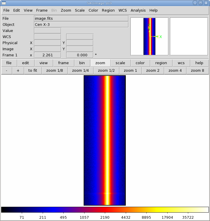
- Click the "Run" button on the lower left corner of the evselect GUI. The image will be displayed automatically in a ds9 window.
The image can be displayed in ds9 and is shown in Figure 4. The source is centered on RAWX=37; we will extract this and the 10 pixels on either side of it.
- Enter the filtering criteria in the "Selection Expression" area at the top of the xmmselect window: (FLAG==0) && (PI in [500:15000]) && (RAWX in [27:47]).
- Click the round button next the PI column on the xmmselect GUI
- Click on "OGIP Spectrum".
- In the "General" tab, check keepfilteroutput and withfilteredset. In the filteredset box, enter the name of the event file output. We will use pn_filt_source_WithBore.fits.
- In the "Spectrum" tab, set the file name and binning parameters for the spectrum. Confirm that withspectrumset is checked. Set spectrumset to the desired output name. We will use source_pi_WithBore.fits. Confirm that withspecranges is checked. Set specchannelmin to 0 and specchannelmax to 20479.
- Click "Run".
For the background, the extraction area should be as far from the source as possible. However, sources with > 200 ct/s (like our example!) are so bright that they dominate the entire CCD area, and there is no source-free region from which to extract a background. (It goes without saying that this is highly energy-dependent.) In such a case, it may be best not to subtract a background. Users are referred to Ng et al. (2010) for an in-depth discussion.
While this observation is too bright to have a good background extraction region, we will note for the sake of demonstration that a background spectrum can be extracted following the same method, setting the region to an area as far from the source as possible. For our example data, the "Selection Expression" be (FLAG==0) && (PI in [500:15000]) && (RAWX in [3:5]), the output filtered event file be pn_filt_bkg.fits, and the spectrum bkg_pi.fits.
Check for Pile Up
Depending on how bright the source is and what modes the EPIC detectors are in, event pile up may be a problem. Pile up occurs when a source is so bright that incoming X-rays strike two neighboring pixels or the same pixel in the CCD more than once in a read-out cycle. In such cases the energies of the two events are in effect added together to form one event. Pile up and how to deal with it are discussed at length here and here, respectively, and users are strongly encouraged to refer to those sections. Briefly, we deal with it in PN TIMING data essentially the same way as in IMAGING data, that is, by using only single pixel events, and/or removing the regions with very high count rates, checking the amount of pile up, and repeating until it is no longer a problem.
To check for pile up, invoke epatplot. Then,
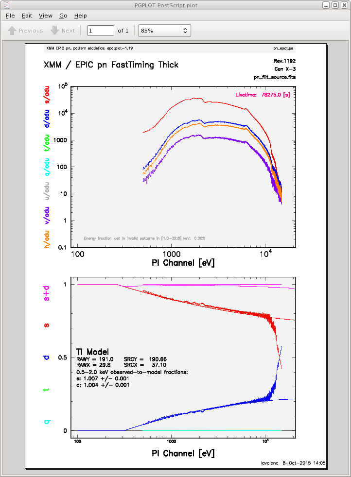
- In the "0" tab, enter the name of the event file that was made when the spectrum was extracted, pn_filt_source_WithBore.fits, the set text box. We want to send the output to a postscript file, so set useplotfile to yes, and enter the file name in the plotfile box. We will use pn_epat.ps.
- In the "1" tab, set withbackgroundset to yes and enter the name of the event file that was made when the background spectrum was made, pn_filt_bkg.fits.
- Click "Run".
The output is shown in Figure 5. In the lower plot, we can see that there is a large difference between the modeled and observed single and double pattern events, and that the observed-to-model fraction for doubles is over 1.0, indicating that the observation is piled up.
My Observation is Piled Up! Now What?
There are a couple ways to deal with pile up. First, you can use event file filtering procedures to include only single pixel events (PATTERN==0), as these events are less sensitive to pile up than other patterns.
You can also excise areas of high count rates, i.e., the boresight column and several columns to either side of it. (This is analogous to removing the inner-most regions of a source in IMAGING data.) The spectrum can then be re-extracted and you can continue your analysis on the excised event file. As with IMAGING data, it is recommended that you take an iterative approach: remove an inner region, extract a spectrum, check with epatplot, and repeat, each time removing a slightly larger region, until the model and observed pattern distributions agree.
To extract only the columns to either side of the boresight, use the procedure shown above:
- Enter the filtering criteria in the "Selection Expression" area at the top of the xmmselect window: (FLAG==0) && (PI in [500:15000]) && (RAWX in [27:47]) &&! (RAWX in [29:45])
- Click the round button next the PI column on the xmmselect GUI
- Click on "OGIP Spectrum".
- In the "General" tab, check keepfilteroutput and withfilteredset. In the filteredset box, enter the name of the event file output. We will use pn_filt_source_NoBore.fits.
- In the "Spectrum" tab, set the file name and binning parameters for the spectrum. Confirm that withspectrumset is checked. Set spectrumset to the desired output name. We will use source_pi_NoBore.fits. Confirm that withspecranges is checked. Set specchannelmin to 0 and specchannelmax to 20479.
- Click "Run".
Be aware that if you do this and are using SAS v. 13.x or older, you will need to use a non-standard way to make the ancillary files (ARFs) for your spectrum! This is discussed further in a later section.
Determine the Spectrum Extraction Areas
Now that we are confident that our spectrum is not piled up, we can continue by finding the source and background region areas. (This process is identical to that used for IMAGING data.) This is done with the task backscale, which takes into account any bad pixels or chip gaps, and writes the result into the BACKSCAL keyword of the spectrum table. To find the source and background extraction areas, call backscale and then
- In the "Main" tab, enter the name of the spectrum, source_pi_NoBore.fits.
- In the "Effects" tab, confirm that withbadpixcorr is checked, and enter the name of the event file, pn_filt.fits, in badpixlocation.
- Click "Run".
Follow the same steps to find the background spectrum area, changing the input spectrum file to bkg_pi.fits.
Create the Photon Redistribution Matrix (RMF) and Ancillary File (ARF)
If you are using SAS v. 14 or higher, making the RMF and ARF for PN data in TIMING mode is exactly the same as in IMAGING mode, even if you had to excise piled up areas.. This is a change from earlier SAS versions; if you are working with an older SAS, you will need to use the special recipe below to generate the ARF (the method to make a RMF file is the same as shown here.)
To make the RMF, call rmfgen from the SAS GUI and then
- In the "main" tab, set rmfset to the output file name. We will use source_rmf_NoBore.fits. Set the spectrumset parameter to the spectrum, source_pi_NoBore.fits.
- Click "Run".
To make the ARF (with SAS v. 14 or higher), call arfgen from the SAS GUI and then
- In the "main" tab, set arfset to the output file name. We will use source_arf_NoBore.fits. Set the spectrumset parameter to the spectrum, source_pi_NoBore.fits.
- In the "detector map" tab, use the pull-down menu to set the map type to psf.
- In the "calibration" tab, set withrmfset to yes and rmfset to source_rmf_NoBore.fits.
- In the "effects" tab, verify that withbadpixcorr is checked, and set badpixlocation to the event file, pn_filt.fits.
- Click "Run".
If you excised regions to make a spectrum and are using SAS v. 13.x or older, you will need to make an ARF for the full extraction area, another one for the piled up area, and then subtract the two to find the ARF for the non-piled regions. To get those, we will need the spectra of the full extraction area and the excised area. We already have it for the full extraction area, so for the excised area, use the same procedure as above, but change the "Selection Expression" to (FLAG==0) && (PI in [500:15000]) && (RAWX in [29:45]), set the filteredset parameter to pn_filt_source_Excised.fits, and spectrumset to source_pi_Excised.fits.
Now we can use the spectra to make the ARFs. Invoke arfgen from the SAS GUI, and then
- In the "main" tab, set arfset to the output file name. We will use source_arf_WithBore.fits. Set the spectrumset parameter to the spectrum, source_pi_WithBore.fits.
- In the "detector map" tab, use the pull-down menu to set the map type to psf.
- Click "Run".
Use the same procedure to make the ARF for the excised region, changing the arfset parameter to source_arf_Excised.fits and spectrumset parameter to source_pi_Excised.
We can now subtract them. This is easiest to do on the command line:
addarf "source_arf_WithBore.fits source_arf_Excised.fits" "1.0 -1.0" source_arf_NoBore.fits
The spectrum can be fit using HEASoft or CIAO packages, as SAS does not include fitting software.
If you have any questions concerning XMM-Newton send e-mail to xmmhelp@lists.nasa.gov