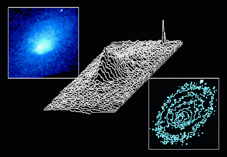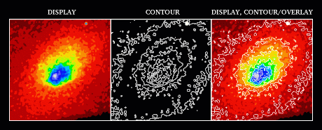
General PlottingAfter reading in data with the READ_IMAGE command, XIMAGE can display it as an image with the DISPLAY command, as a pseudo-3D surface with the SURFACE command, or as contour lines with the CONTOUR command.
ColorsThe colors used by the display are defined via a color table. At the ximage startup, a default color table is set, however it may be changed with the CCT command. The syntax "CCT [colortable]" changes the colors in the current displayed image while "CCT/SET [colortable]" makes that color setting the default color table. The default color table will be used in any subsequent plot, while the color table from "CCT [colortable]" is only used in the current displayed image. The SHOW command prints the current default and displayed color tables:
  Displayed Color Table : bluebase1( Brightness = 0.5, Contrast = 1.0 )
  Default Color Table   : bluebase1( Brightness = 0.5, Contrast = 1.0 )
For a list of all available color tables and how they look, see the Color Tables page. The CCT command behaves differently depending on the color capabilities of the PGPLOT device. Basically there are two types of devices, which we will refer to as dynamic-color and static-color. With dynamic-color devices, the color table can be changed for a currently displayed image (CCT [colortable]), while color-static devices keep the colors they are originally plotted with. To make color adjustments to a static-color device, the color table must be set (CCT/SET [colortable]) before displaying the image.
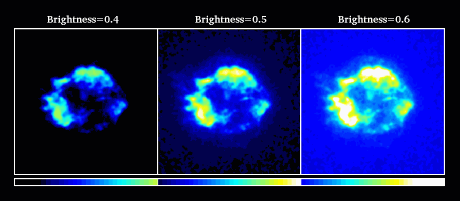
If your display is limited to 256 colors (8-bit), you have a PseudoColor display. Owners of this type of display often experience color-flashing when switching between applications which use many colors. The benefit of this type of display is that you can use commands such as CCT/LOOP to quickly try out available color tables. Color tables can be further modified by brightness and contrast values applied to them. Brightness increases from 0.0 to 1.0 with a default value of 0.5. Decreasing the brightness shifts the colors in the scale to the right, while increasing the brightness shifts them to the left. Use CCT's BRIGHTNESS qualifier to change the brightness.
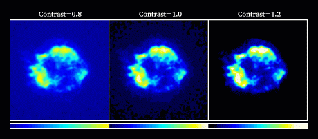
Contrast defaults to 1.0, with possible values ranging over all real numbers. Increasing the contrast compresses the color scale, while decreasing it stretches the color scale. Negative contrast values flip the direction of the color table. Use CCT's CONTRAST qualifier to change the contrast.
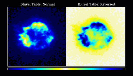
A quick way to reverse a color table is to use CCT's REVERSE qualifier, which sets CONTRAST=-CONTRAST and BRIGHTNESS=1.0-BRIGHTNESS.
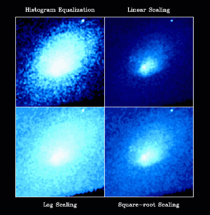
Note that brightness and contrast adjustments must be set with the SET qualifier before displaying an image on a static-color device. Setting the color of contours and surfaces is a simpler than images. When plotting them, set the desired color index with CONTOUR/COLOR=n or SURFACE/COLOR=n. The color indices 0-15 are recommended. See the PGPLOT Quick Reference for the default definitions of these reserved color indices. To see all currently defined colors, including those set by the current color table, plot the color legend to a displayed image with the COLORS/PLOT command. ScalingThe scaling used in displaying an image can dramatically affect its appearance. By default the histogram equalization is used, however linear, logarithmic and square-root scaling are available through DISPLAY's LINEAR, LOG, and SQRT qualifiers, respectively.
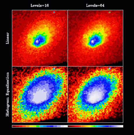
The best scaling to use depends on the character of the image data. Histogram equalization works well with most distributions, as it maps pixels into color bins such that each color is used to draw about the same number of pixels. For low count images, however, there aren't enough unique pixel values to fill up the available colors. Linear scaling is useful for data values which are evenly distributed and with a relatively small range, while logarithmic and square-root scaling are better for data values with a large range. These scalings are also available with the CONTOUR command, however, the SURFACE command only provides linear scaling by default and logarithmic scaling with the LOG qualifier. Number of LevelsDepending on the scaling selected and the distribution of data values, XIMAGE calculates a set of levels. Pixel values less than or equal to the first level are plotted with the first color, values less than or equal to the second level but greater than the first level are plotted with the second color, and so on. By default the number of levels is set to 16, however, LEVELS/NUM=n may be used to change the number of levels calculated. Increasing the number of levels increases the number of colors plotted, resulting in smoother images.
For images where the number of unique pixel values is relatively low, changing the number of levels can have an extreme effect on the histogram equalization scaling. When there are more levels than unique pixel values to fill them, the image can become too dark because colors in the upper range of the scale are unused. In this case, a lower number of levels should be set.
ViewportsThe viewport is the region of the display where an image is plotted. By default a large viewport in the center of the device is used.A common method for getting two images on a page has been to use DISPLAY/LEFT followed by DISPLAY/RIGHT/OVERLAY, however, viewport configuration files (VPC) allow a variety of image placements. VPCs are defined as a list of viewports in a text file, usually ending with the extension ".vpc". The command "VIEWPORT [VPC file]" sets up XIMAGE such that subsequent calls to the DISPLAY, CONTOUR, and SURFACE plot to the viewports in the order defined in the VPC. For example, the command "VIEWPORT 3x1" (.vpc can be omitted) was used in the graphic below.
Note that the effects of OVERLAY and NOFRAME are active when a VPC is set. Although for CONTOUR, OVERLAY has a special meaning in this circumstance. The OVERLAY qualifier stops the advancement of the viewport so that contour lines are plotted on top of the current image. For a list of all available viewport configurations, see the Viewport Configurations page.
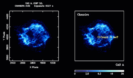
LabellingXIMAGE provides many ways to label images. The left image demonstrates the default labelling, while the right image utilizes special labelling commands.
By default, the field name, instrument and exposure time are printed over the image, as in the left image. To blank out the field name (i.e. the upper title), use the command TITLE " " before displaying an image. To blank out the instrument and exposure time (i.e. the lower title), use the command TITLE/LOWER " ". To revert back to the standard behavior, use the command TITLE/RESET. Titles are automatically reset when a new image is read in. It is also standard to have the axes labelled with detector coordinates, a feature that can be turned off by using the NOFRAME option with DISPLAY. The VPLABEL command plots labels with respect to the viewport, and is recommended when labelling an entire image. For example, the "CAS A" label, is the result of VPLABEL/BOTTOM/JUST=RIGHT "CAS A". The outside of the viewport is labelled by default, however, a negative value for the MARGIN option will place the label inside the viewport as with the "Chandra" label. The LABEL command primarily labels points specified in detector coordinates, and is recommended when indicating specific points in the image as with the "Could it be?" label. A color scale like the one at the bottom of the right image is plotted by running the SCALE command after plotting an image. If a viewport configuration file is in effect, the commands SCALE and VPLABEL will label the collective area of all the viewports, unless you use SCALE/CURVP or VPLABEL/CURVP which forces the labelling of the current viewport.
Please send reports of errors to : xanprob@athena.gsfc.nasa.gov HEASARC Home | Observatories | Archive | Calibration | Software | Tools | Students/Teachers/Public Last modified: Wednesday, 27-Aug-2025 14:25:47 EDT |


