Using SCORPEON Models in XSPEC

Overview

The NICER SCORPEON background model is a new background modeling technique. Unlike other models, SCORPEON produces an adjustable background model which can be fit within XSPEC just like the source spectral model. This page describes how to use the results of SCORPEON within XSPEC.

Read this thread if you want to: Use SCORPEON Background Models

Last update: 2024-02-27

Introduction

The NICER X-ray Timing Instrument is non-imaging instrument. This means that for most work, both in spectroscopy and light curve analysis, the background must be subtracted based on an a priori model. As of NICERDAS version 10 (HEASoft 6.31 and later), three backgrond models are included in NICER's software and calibration suite. This page discusses the SCORPEON model and how to use the SCORPEON background models within XSPEC.

Like all NICER background models, the SCORPEON model attempts to estimate the background which would apply to a specific spectrum. Various training variables, such as COR_SAX, overshoot count rates, undershoots, etc. are used to make an a priori estimate of the background contributions of each component.

As described on the SCORPEON Overview page, there are many background components included within SCORPEON, some of which are due to the X-ray background and some of which are due to non-X-ray background terms such as high energy electrons and cosmic rays. Based upon the limited training variables, SCORPEON is not able to provide an independent estimate of all components.

Indeed, there is ambiguity between several of the components, especially the electron-dominated components: for the same level of overshoot counts, the three electron-dominated SCORPEON background components have nearly three orders of magnitude difference in in-band count rate.

Because of this, a priori NICER background modeling will always be imperfect to some extent. This statement applies to all NICER background modeling, including SCORPEON, 3C50 and Space Weather. There simply are not enough training variables to constrain all possible background variability.

However, SCORPEON has an additional capability that other background models do not. The output of SCORPEON is an adjustable model that can be fit and manipulated within XSPEC.

This capability has several major advantages:

• Over- and under-subtraction is rarely a problem; the background can be adjusted to resolve such problems
• With a better background fit, NICER becomes more sensitive to faint targets and spectral features
• Uncertainties in background model parameters can be determined simultaneously with the uncertainties in the scientist's science parameters; i.e. the uncertainty in science parameters more accurately reflects the uncertainty in the background

A unique feature of using the SCORPEON model is that you are not subtracting the background, you are modeling it along with your source.

However, this approach does have some negative impacts. An adjustable background model that must be fit in XSPEC means more work for the analyst. Using a SCORPEON model is not a simple matter of background subtraction, but rather an additional fitting step as well as some need for the analyst to understand the origins of NICER background.

Also, adjusting and fitting a SCORPEON background may be infeasible when the scientist is working with a large scale analysis pipeline, or if data must be shared with an analyst that does not use XSPEC. In those cases, SCORPEON does provide an option to produce a background file, similar to the way that the 3C50 and Space Weather models operate. This background file will be simply subtracted from the data by XSPEC and is not adjustable.

In this thread, we will discuss the following topics

• Review how to generate a SCORPEON estimate
• Demonstrate how to load NICER data with a SCORPEON background model into XSPEC
• Loading multiple spectra
• Assigning a source model
• Fitting source and background parameters
• Guidelines and things to watch out for

Producing a SCORPEON Background Model

There are several ways to produce a SCORPEON background model. In short, the NICER-recommended way is to use the nicerl3-spect task. This task produces all spectral products, including spectrum, responses, and background estimates. The user can control various aspects of the product generation, including which background model to apply. For more information and options, please see the SCORPEON Overview page.

In this example, we will process a fictional observation 2010100101. For the example, we will download the data into the directory /path/to/data/2010100101 and process it with nicerl2. Then we will run nicerl3-spect to generate spectral products. First, we will change to the working directory where the observation resides. cd /path/to/data And then we will run nicerl3-spect. nicerl3-spect 2010100101 clobber=YES bkgmodeltype=scorpeon Here 2010100101 is the observation directory name; you would substitute your own observation. We have also explicitly set bkgmodeltype=scorpeon to select the SCORPEON model (although that is the default). For more variations on using nicerl3-spect, please see the nicerl3-spect Thread.

After running the nicerl3-spect task, there are a number of outputs placed in the 2010100101/xti/event_cl directory, including:

• ni2010100101mpu7_sr.pha - source+background spectrum
• ni2010100101mpu7.arf - source ARF response
• ni2010100101mpu7.rmf - source RMF response
• ni2010100101mpu7_bg.xcm - SCORPEON background model
• ni2010100101mpu7_bg.rmf - background RMF response
• ni2010100101mpu7_sk.arf - diffuse sky ARF response
• ni2010100101mpu7_load.xcm - "load" file for convenience

Here we used the default output file names, although it is possible to change these. If you have a different workflow, you will have to generate your own spectrum and responses manually using extractor or niextspect, and produce background files manually using niscorpspectmod (see Manually Estimating NICER Backgrounds for more information), and take note of whichever file names you produced.

The "Load" Script and Loading Data Into XSPEC

The "load" file is a convenience XSPEC script which loads data, responses and backgrounds into XSPEC so that you are ready to begin analysis.

Let's examine what is in this load file. We will use the Unix "cat" command to list a file's contents: cat 2010100101/xti/event_cl/ni2010100101mpu7_load.xcm The contents should look something like this: data 1:1 2010100101/xti/event_cl/ni2010100101mpu7_sr.pha ignore bad resp 1:1 2010100101/xti/event_cl/ni2010100101mpu7.rmf arf 1:1 2010100101/xti/event_cl/ni2010100101mpu7.arf set nicer_bkgspect 1 @2010100101/xti/event_cl/ni2010100101mpu7_bg.xcm As you can see, we load "data", "resp"onse and "arf" responses just like any XSPEC analyst would. There is absolutely no difference between what is shown here and what is used for SCORPEON modeling. However, the SCORPEON steps that happen next are different.

The "set nicer_bkgspect 1" command sets an XSPEC (TCL) variable to indicate to the background script which spectrum number this will apply to. If you are just fitting one spectrum, this number will always be "1" but if you have multiple spectra (see next sections), you may have different numbers.

Finally, the "@2010100101/xti/event_cl/ni2010100101mpu7_bg.xcm" tells XSPEC to execute the SCORPEON background model statements. This is a large file that defines NICER background model templates as well as setting a priori parameter norms. We will get more into these in later sections.

Summary for One Spectrum

In summary, to load data into XSPEC you can use the nicerl3-spect "load" script or you can design your own load process. First you load the data into spectrum number 1 into datagroup 1. data 1:1 myfile.pha resp 1:1 myfile.rmf arf 1:1 myfile.arf and then we load the SCORPEON background model. set nicer_bkgspect 1 @myfile-bkg.xcm where myfile* could be any of your spectral products.

Multiple Spectra

Neither XSPEC nor SCORPEON are limited to just one spectrum. Users often have multiple datasets loaded into XSPEC, either joint fitting between observatories or fitting multiple NICER data sets simultaneously. Either way, this is supported. Here we give an example of loading two NICER spectra: data 1:1 myfile1.pha resp 1:1 myfile1.rmf arf 1:1 myfile1.arf set nicer_bkgspect 1 @myfile1-bkg.xcm data 2:2 myfile2.pha resp 1:2 myfile2.rmf arf 1:2 myfile2.arf set nicer_bkgspect 2 @myfile2-bkg.xcm Here we have used the shorthand myfile1 for the first spectrum and associated products, and myfile2 for the second spectrum and products. The only real difference is that for the second spectrum we set "nicer_bkgspect" to a value of "2" to tell SCORPEON to apply the second background to the second spectrum.

Jointly Fitting Spectra from Different Observatories

Fitting multiple spectra from different observatories is really no different than fitting multiple spectra from NICER alone. SCORPEON can be used in this case.

Users often have multiple datasets loaded into XSPEC, either joint fitting between observatories or fitting multiple NICER data sets simultaneously. Either way, this is supported. Let's provide an example with NuSTAR and NICER, which is a common combination: data 1:1 nustar_sr.pha resp 1:1 nustar.rmf arf 1:1 nustar.arf back 1 nustar_bk.pha data 2:2 myfile2.pha resp 1:2 myfile2.rmf arf 1:2 myfile2.arf set nicer_bkgspect 2 @myfile2-bkg.xcm Here we have used the shorthand that "nustar" is the name of the spectrum and its associated spectral products, as produced by nupipeline and/or a NuSTAR background estimator. The NICER data is loaded as the second spectrum (and second data group) using the shorthand notation myfile2.

What do the numbers mean in data / arf / response statements?

In the discussions above, we are using the XSPEC data, background, response and arf statements to load in various files. Each of these statements has one or more numbers attached to it. What do they mean? Let's review these statements. data 1:2 nicer1.pha back 2 nicer1_bk.pha

The first number of the data statement is the data group number that the spectrum is a member of. In this example, we have placed nicer1.pha in the 1st data group. Each data group has its own set of spectral parameters. Typically, although not always, you will want to place each spectrum file into a different data group, so that you can allow total intensities to vary between spectra etc. It is common to use the notation "data 1:1 file1.pha, 2:2 file2.pha" and spectrum 1 will be placed into data group 1, spectrum 2 into data group 2.

The second number of the data statement (and only number of the background statement) is the spectrum number. This is how you refer to each loaded spectrum file. Here we have loaded nicer1.pha as spectrum number 2. For the background statement, the spectrum number should refer to the spectrum that was just loaded using the data statement. resp 1:2 nicer1.rmf arf 1:2 nicer1.arf

The first number of the arf and response statements is the source number. For XSPEC, you can have multple sources that all contribute flux and counts towards a measured spectrum. Note that the source number is NOT the same as the data group or spectrum number. In most basic cases, the source number will be 1.

However, as an example of where multiple sources could be useful, consider a NICER observation of a target that has another X-ray source very nearby inside NICER's field of view. You can use two XSPEC sources, one for each of the known X-ray emitting sources in the NICER field of view, and have a model and response for each.

In fact, the SCORPEON model is implemented as two extra XSPEC sources, sources 98 and 99 by default, which correspond to the non-X-ray background and X-ray backgrounds, respectively. The "bg.xcm" file handles creating these sources and models.

The second number of the response and arf statements is the spectrum number. This spectrum should match the file that was loaded with the "data" statement.

For more reference information on how to use these statments, please see the XSPEC manual.

Using Python

XSPEC has a Python interface known as PyXspec and SCORPEON supports this. When you run nicerl3-spect, set the parameter outlang=python, and the background and "load" scripts will be written in Python rather than XSPEC's xcm language. Please see the nicerl3-spect page for additional information.

Please note that you must have a version of Python that supports PyXspec, and this version must be designated when you build HEASoft.

Starting XSPEC and Loading Data

Let's begin by starting XSPEC xspec Next, we can load our data. We can use the "load" file we generated earlier, @2010100101/xti/event_cl/ni2010100101mpu7_load.xcm where 2010100101/xti/event_cl/ni2010100101mpu7_load.xcm is the name of the load file generated by nicerl3-spect. You can also type the individual commands as typed above.

During the "load" process, a large number of commands will scroll by. This is normal. During this process all SCORPEON's model templates are defined using XSPEC's mdefine statement, and a priori parameter values are set.

Problems Loading? You may encounter problems loading NICER + SCORPEON data into XSPEC. Possible problems:

• Can't find background RMF or sky ARF. Typically this is caused by running XSPEC from a different working directory than when nicerl3-spect was run. You must run both from the same working directory.
• "You must define nicer_bkgspect". Be sure you set nicer_bkgspect each time you load the background model script.

Let's plot the spectrum in XSPEC. We will use the "X" windows plotting device. cpd/xs setplot energy setplot rebin 10 10 plot ldata The "setplot energy" command makes the X-axis of the plot be log(Energy), while the "setplot rebin" command applies light rebinning. The rebining may not be necessary if you used the default grouping parameters when running nicerl3-spect.

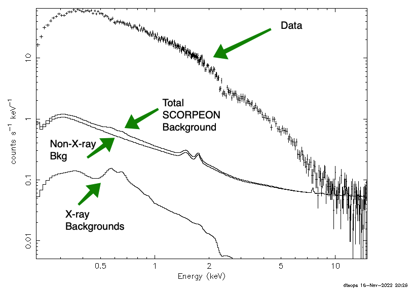
The result for this fictitious observation could look something like this:

The crosses are NICER's source+background measurements, as extracted from the cleaned event files. The lower traces, from the bottom up, are the X-ray background, non-X-ray background and total background estimate.

At this stage all we have is a background model and no source model, so it is not surprising that we don't have a good match between the model and spectrum. Let's remedy that.

Define a Source Model

With any spectral analysis you need to decide how to model the spectrum of your source. This is typically a case-by-case scientific decision. The selection of the model is outside is outside of the scope of this thread. For our purposes we will assume the source can be modeled with an absorbed broken power law or "bknpower" within XSPEC.

We define source models as always, using the "model" command. No change to the syntax is required.

SCORPEON models are also models, but are stored by default as "sources" 98 and 99. As long as you do not explicitly alter those sources, any model commands you type will not interfere with SCORPEON.

Therefore, we will enter the XSPEC model command that includes absorption and a broken power law: model tbabs*bknpower where tbabs is the Wilms et al absorption model and bknpower is the broken power law. Although for your science case you should use your knowledge to set parameters to the good starting values, for our case we will use the default values.

As discussed below, we will use the "pgstat" statistic because most NICER spectra have low counts at high energies where the background is most dominant. statistic pgstat Using this statistic (or "cstat" if applicable) will avoid biases that can distort your background fit due to low counts statistics.

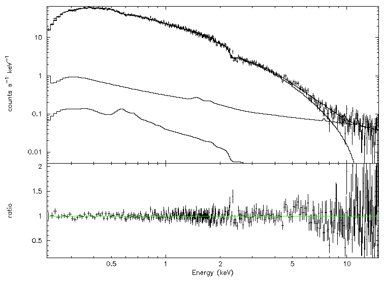
Now, finally, we will type the "fit" command fit to begin simultaneously fitting source and background. If the fit does not converge immediately, we may need to monitor the parameters and make sure none of them are at extreme values. After several iterations of fitting, we arrive at this joint source+background fit.

Here is the resulting fit after typing "plot ldata ratio":

The residuals are quite flat across the entire spectrum and a few percent over most of the range. There appear to be no over- or under-subtractions.

We can use the XSPEC "flux" command to obtain fluxes in a desired energy range (0.5-10 keV in this example). XSPEC12>flux 0.5 10 Source 1 Model Flux 0.029191 photons (9.0728e-11 ergs/cm^2/s) range (0.50000 - 10.000 keV) Source 99 Model Flux 1.1043 photons (6.4913e-09 ergs/cm^2/s) range (0.50000 - 10.000 keV) Source 98 Model Flux 31.293 photons (9.7846e-08 ergs/cm^2/s) range (0.50000 - 10.000 keV) As you can see, the flux for each model component is displayed. Source 1 is our target's X-ray spectrum, and sources 98 and 99 are the X-ray and non-X-ray backgrounds.

Managing SCORPEON Parameters

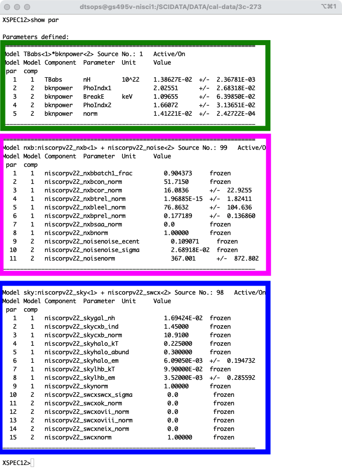
Up until this point, we have been ignoring the SCORPEON parameters. Let's take a closer look. We can use the "show par" XSPEC command to display all of the active parameters. Unlike a normal case, we see large display of values.

The parameters in the green box   at the top are the normal science parameters for whatever model you chose (in this case the absorption and broken pawer law parameters).

The parameters in the magenta/pink box   in the middle are the NXB or "non-X-ray Background" parameters. This source has two model components, "niscorpv22_nxb" and "niscorpv22_noise", which are addative. This entire source is known by it's name, "nxb" and you can set, freeze and thaw the parameters of this source using that name. For example we can freeze parameter 4 of the "nxb" model with the following commands. newpar nxb:4 0.0 freeze nxb:4 As you can see, the notation is simply "nxb:n" where n is a parameter number. For the science target, we don't need to refer to the model by name so you can still refer to those parameters by their simple numerical values.

The parameters in the blue box   at the bottom are the X-ray background terms. This model is known as "sky" to refer to components that are due to the diffuse X-ray sky (local or galactic). There are two components in this model, "niscorpv22_sky" and "niscorpv22_swcx", which are again addative.

Important Note. You should never change or thaw the overall model "norm" values from the default values of 1.0 (nxb:8, sky:9 and sky:15 in the list above). An exception to this rule is the noise peak norm (nxb:11).

What Are the SCORPEON Parameters?

First of all, let's discuss SCORPEON naming. All of the SCORPEON model functions begin with a version number. In the example above, all model functions have the form, niscorpv22_ Which indicates "NI"CER "SCORP"EON "V"ersion 22, followed by a which indicates what SCORPEON components it represents. Here niscorpv22_nxb refers to the Non-X-ray Background components.

As the SCORPEON model is updated, new versions may become available. In principle the user could compare multiple different versions, since they are all available separately.

Each model function has a set of parameters, which we describe briefly here.

SCORPEON "niscorpv22_nxb" Parameters

• batch1_fract - a quantity referring to the fraction of different detector batches that are enabled (batches have consistent background within the batch, but different between batches).
• con_norm - Normalization of the CON (constant non-X-ray background) component (fixed by number of enabled detectors)
• cor_norm - Normalization of the COR (cosmic ray) component (set a priori with an allowed fitting range)
• trel_norm -Normalization of the TREL (trapped electron) component (set a priori with an allowed fitting range)
• leel_norm - Normalization of the LEEL (low energy electron) component (set to zero by default with an allowed fitting range)
• prel_norm - Normalization of the PREL (precipitating electron) component (set to zero but allowed to vary if COR_SAX is less than 1.5)
• saa_norm - Normalization of the SAA (South Atlantic Anomaly) component (set a priori, usually 0)
• norm - do not change from 1.0

SCORPEON "niscorpv22_noise" Parameters

• noise_ecent - noise peak centroid energy [keV] (set a priori, and variable if broad peak detected)
• noise_ewid - noise peak sigma width [keV] (set a priori, and variable if broad peak detected)
• norm - noise peak count rate (set a priori, and free to vary)

SCORPEON "niscorpv22_sky" Parameters

• gal_nh - nH of galactic emission (set a prioriy based on "nh" tool)
• cxb_ind - power law index of cosmic X-ray background (fixed at Capelutti et al. 2017 value)
• cxb_norm - norm of cosmic X-ray background [photons/s/keV/cm²/sr] (set a priori at Capelutti et al. 2017 value with an allowed fitting range)
• halo_kT - temperature of galactic halo (fixed at Kaaret et al. 2019 value)
• halo_em - emission measure of galactic halo (set a priori based on Kaaret et al. 2019 model but allowed to vary +/- 50%)
• lhb_kT - local hot bubble temperature (fixed at Liu et al 2017 value)
• lhb_em - local hot bubble emission measure (set a priori based on Liu et al. 2017 value but allowed to vary +/- 50%)
• norm - do not change from 1.0

SCORPEON "niscorpv22_swcx" Parameters

• swcx_sigma - overall broadening for all SWCX lines (fixed at 0.0)
• ok_norm - norm of neutral oxygen K line [photons/s/cm²/sr] (fixed at zero)
• ovii_norm - norm of SWCX O VII line [photons/s/cm²/sr] (fixed at zero)
• oviii_norm - norm of SWCX O VIII line [photons/s/cm²/sr] (fixed at zero)
• neix_norm - norm of SWCX Ne IX line [photons/s/cm²/sr] (fixed at zero)
• norm - do not change from 1.0

SCORPEON XSPEC Guidelines

Here we provide some important and basic guidelines for SCORPEON work within XSPEC. Following these guidelines will provide the best results for your analysis.

Use a Wide Energy Range

Use as wide an energy range as possible (0.22-15 keV). Even if your target is detectable in a narrow energy range, the background components have different broadband spectra.

Using the entire energy range helps SCORPEON distinguish between components.

Use one of the following commands: ignore bad # or ignore **-0.22,15.0-**

Use Poisson Statistics

Use the Poisson statistics ("cstat" or "pgstat") during fitting. Even when your target has a large number of counts in a certain energy band, the counts above 10 keV are typically very low.

Using Poisson statistics avoids biases that can distort the background fit.

You can enable Poisson statistics with one of the following commands: statistic pgstat # or statistic cstat

Ignoring Low Energies?

Normally, we recommend that you include the full NICER energy range during fits with SCORPEON models. However, you may be forced to ignore low energy channels. For example, because of a highly absorbed source, the spectrum may be systematics-dominated at low energies and add nothing to your fit. In that case, you can ignore low energies, but you should be aware of some changes you should apply to the fitting process.

If you are ignoring low energy portions of a spectrum with a SCORPEON model, you should freeze some parameters so that those model components do not become unphysical.

If you ignore 0.5 keV and below, freeze the noise_norm, lhb_em and gal_nh parameters.

If you ignore 1.0 keV and below, also freeze the halo_em parameter.

Check for artifacts

Check for known artifacts that indicate you should adjust how the background is modeled. A more detailed background artifact page is in development.

Know that SCORPEON parameters have sensible defaults

As much as possible, SCORPEON components are parameters are physically-motivated and have physically-motivated parameter values and minimum-maximum parameter ranges.

By default, the SCORPEON model that is produced for your data set will have some parameters fixed and some parameters allowed to vary. Unless you have good reason, you should not thaw frozen parameters or change the min/max ranges. The ranges and thawed/fixed settings for each parameter are custom tailored to your observational conditions.

In many cases, parameter values are frozen at the values as determined by published literature (for example, CXB power law index, galactic halo temperature, local hot bubble temperature).

In other cases, the SCORPEON model provides an estimate as well as an estimated range for the parameters, which are based on published literature or based on measurements taken from NICER background observations.

In some cases, such as precipitating electrons (PREL) or the South Atlantic Anomaly (SAA) components, a parameter may be thawed only if NICER passes through the relevant geographic regions where these components are active.

In almost every case, the NICER team has attempted to provide sensible and motivated parameter values and ranges. You should be able to type "fit" in XSPEC without being too concerned that parameters will become unphysical.

There are some exceptions to this general guideline.

Generally speaking the precipitating electron (PREL) component can be highly variable over many orders of magnitude, but only in a very small polar horn geographic region where COR_SAX < 1.5. SCORPEON is currently unable to predict the contribution of this component with high accuracy. When SCORPEON detects that NICER is passing through a region where PREL is potentially active, it sets the normalization to zero but allows it to vary over a wide range.

The Low Energy Electron (LEEL) background component is similar, except that it can appear anywhere in the NICER orbit, not just the polar horn regions. Thus, this parameter is always allowed to be free over a wide range.

Saving Your Work With "save"

You can save your XSPEC work session using the "save" command. For example, save all mysession.xcm will save all data, response, background, model and parameters to the named file. As of HEASoft 6.31, XSPEC supports the save command properly with SCORPEON models. If you try to work with NICER + SCORPEON data in HEASoft 6.30, you may encounter some problems with the "save" command, and for this reason we don't recommend using older versions of HEASoft.

Modifications

• 2022-11-30 - initial draft
• 2023-01-04 - added fitting guidance; some formatting improvements
• 2023-07-07 - add discussion of jointly fitting multiple observatories; discussion of the numbers in "data" statements, etc