Simulation of an Xtend Spectrum, Including the Background Components
Non X-ray and X-ray Background Components
Xtend signals include charged particle events.
Most are identified by the charge distribution of 3x3 or 5x5 event pixels and are removed by screening.
However, some particle events remain in the screened (cleaned) data as noise or so-called non-X-ray background (NXB).
The night Earth observations, when the telescope points at the Earth's night surface, provide a good proxy
to evaluate this background. The data are compiled in a public database to assess the NXB level during observations.
The Xtend instrument team studied NXB data obtained during the commissioning and
early PV observations and formulated a model to describe the spectrum used successfully
in the published PV-phase results.
Xtend observation proposers must assess the contribution to justify the proposed observations.
This web page instructs how to include the NXB component in a spectral simulation.
The model does not include a sky X-ray background like the cosmic X-ray background (CXB).
This page instructs how to include the component, too.
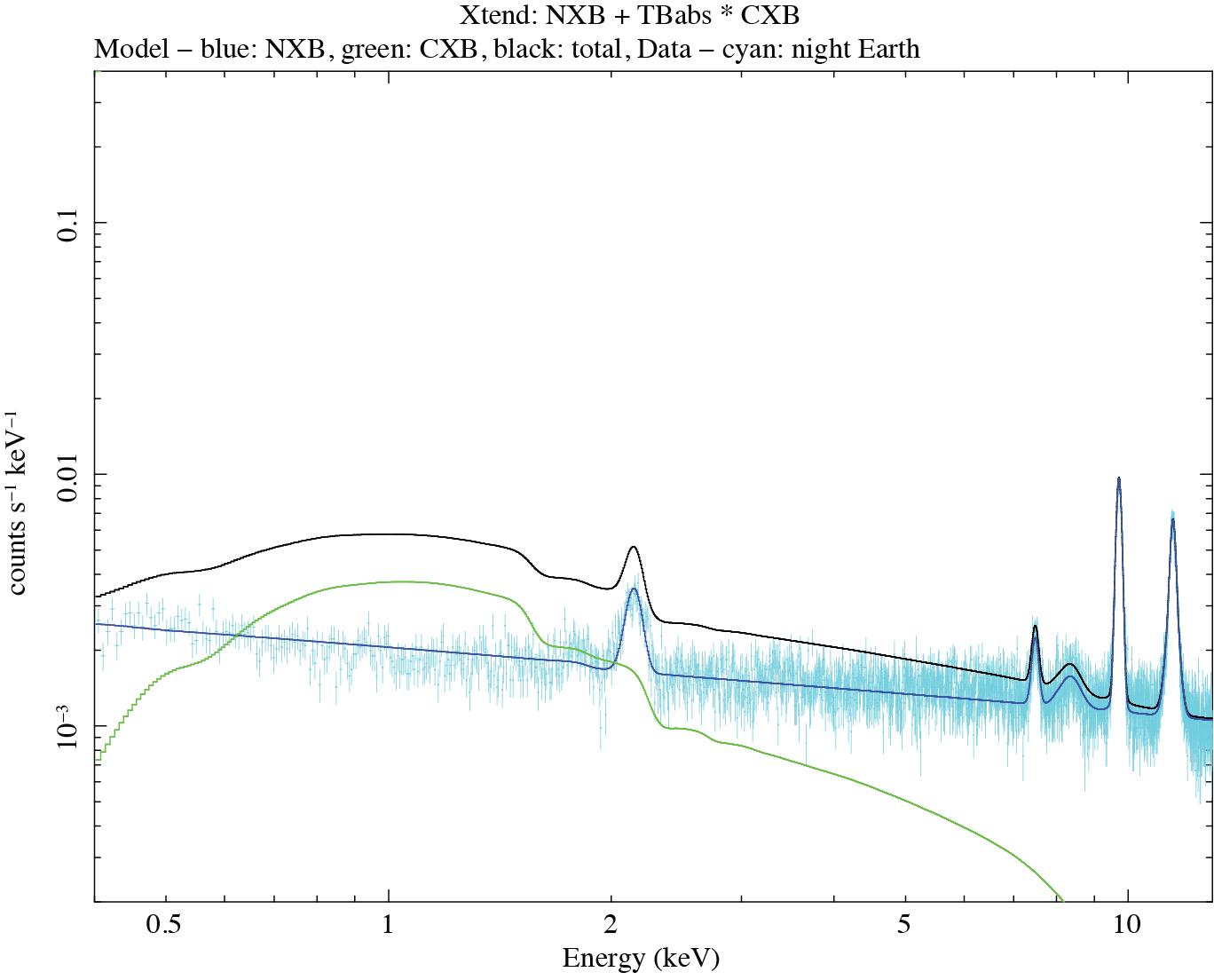
The plot below shows the typical NXB and CXB spectra with Xtend.
The CXB dominates the contribution in the soft band, while it is less than a quarter of the NXB above ~5 keV.
Xtend night-Earth spectrum (cyan), NXB model convolved with the diagonal response matrix (blue),
and CXB spectrum model in Boldt 1987 (green)
attenuated by a NH = 10-21 cm-2 absorber and
convolved with the Xtendrmf and a flat arf response file.
The data ard models are normalized for a r = 2.5' encircled area.
The current NXB data
considers X-ray grade (02346) events extracted from 360 < DETY < 1440, excluding rows with Fe55 calibration source events,
which is equivalent to 1081 (arcmin)2 in the sky.
The NXB intensity depends on the ACTY coordinates and the observatory's particle environments, which should be less than ~50%.
You can, therefore, produce an NXB spectrum for your source spectrum by normalizing the NXB spectrum with the extracting region's
areal scale.
There are two methods of simulating a spectrum with the NXB using Xspec.
One is to include the NXB in an input model, and the other is to feed the NXB spectrum FITS file into Xspec,
downloadable from the proposal preparation page.
The latter is conventional and straightforward,
while the former can be easily adjustable to different source sizes or complicated cases.
The following example assumes spectral simulation of a point source using an on-axis point source arf.
It also applies to extended source simultation if users have an appropriate extended source arf.
However, the extended source arf depends strongly on their spatial distribution,
so those who propose extended sources are encouraged to use HEASim or another detector simulator.
The tool should naturally have a function that includes the NXB or sky background components.
Method 1: Include the NXB in an Input Model
You first launch Xspec from a command line.
terminal> xspec
This method links each input model component to a response file, for which you must input a response file into Xspec by design.
To input a response file, you must input a source spectrum before inputting the response file.
Of course, you do not have one yet, so we here input the NXB file as a dummy.
The simulation does not use the spectral information in the source file,
so technically, the source spectrum file can be any ungrouped Xtend spectrum.
After that, you input the corresponding response and ARF files.
The NXB model uses the diagonal matrix,
xtend_nxb.rmf,
so you input two sets of response files.
The first number of each response or arf statement is the model ID,
which you assign when inputting each model.
Here, we assign 1 to the source model and 99 to the NXB model. Note that the first number
of the data command has a different meaning: it is the data group number.
A detailed explanation of the option is in the Xspec manual and
the NICER SCORPEON page.
We choose an absorbed thermal (TBabs * apec) spectrum at a temperature of 2 keV as a source spectrum.
The number after the model command corresponds to the model ID.
The NXB model has many parameters. You can download xtd_nxb_ave_R2p5_2025.xcm
and load it into Xspec.
XSPEC> @xtd_nxb_ave_R2p5_2025.xcm
This xcm file is the same as xtend_nxb_average.mo on the
NXB spectral models page, except for two things.
One is that it assigns the model to model ID 99.
Edit the file if you choose a different model ID.
As described above, you must load this file after the command "response 99:1 ..."
or you will get an error message stating, "XSPEC Error: no corresponding source exists for model source number."
Two is that the area scale parameter det:1 is adjusted to 0.01816 for an r = 2.5 arcmin encircled extraction region.
If you simulate a different region size, calculate the areal scale to 1081 arcmin2 and input it as
XSPEC> newpar det:1 areal_scale
By typing the following commands, you can dump
(the current setup) and view the model in a plot.
XSPEC> show all
XSPEC> setplot device /xw
XSPEC> setp e
XSPEC> setplot com r x 0.4 12.0
XSPEC> setplot com r y 3e-4 0.6
XSPEC> plot ldat
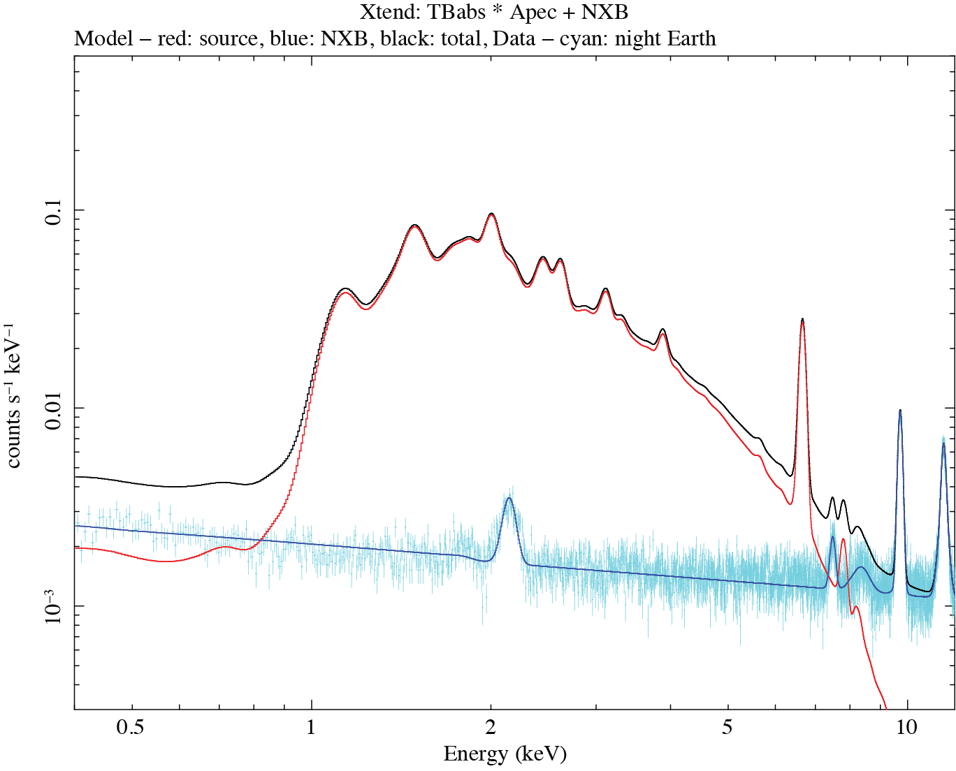
Simulation model (TBabs * Apec + NXB).
Then, let's simulate a spectrum for a 200 ksec exposure with the fakeit command.
XSPEC>fakeit
Use counting statistics in creating fake data? (y):
Input optional fake file prefix:
Fake data file name (xtd_nxb_ave_R2p5_2025.fak): xtd_src_nxb_R2p5_2025_exp200ks.fak
Exposure time, correction norm, bkg exposure time (95611.0, 1.00000, 1.00000): 200000, 1.0, 0.0
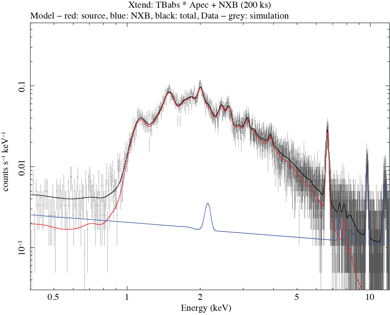
Simulated spectrum of the apec + NXB model for 200 ksec.
Xspec outputs a source spectrum file with the name xtd_src_nxb_R2p5_2025_exp200ks.fak.
You can use this spectrum to evaluate parameter error ranges with the input model.
You can also plot a background-subtracted spectrum by feeding the NXB background spectrum as background with the background command.
XSPEC> backgrnd 1 xtd_nxb_average_R2p5.pha
Method 2: Input the NXB File as Background
You launch xspec and input a spectral model. Here, we assume the same spectral model as the previous method.
Then, run the fakeit command with the NXB file in the argument.
XSPEC12>fakeit xtd_nxb_average_R2p5.pha
For fake spectrum #1 response file is needed: xtd_2025.rmf
...and ancillary file: xtd_ptaimpt_R2p5_2025.arf
Use counting statistics in creating fake data? (y):
Input optional fake file prefix:
Fake data file name (xtd_2025.fak): xtd_src_nxb_R2p5_2025_bgdsbt_exp200ks.fak
Exposure time, correction norm, bkg exposure time (5.26385e+06, 1.00000, 5.26385e+06): 200000, 1.0, 5e7
The command produces source and background files, xtd_src_nxb_R2p5_2025_bgdsbt_exp200ks.fak and xtd_src_nxb_R2p5_2025_bgdsbt_exp200ks_bkg.fak.
You can use them to make a net spectrum.
Background-subtracted spectrum of the TBabs * apec + NXB model for 200 ksec.
Adding X-ray Background or Foreground Sources to the Model
You can also add surrounding point sources or extended foreground or background sources
to the model and assess their contributions. Their models must be linked to the corresponding response files
for simulation, so you must input the files and models in the same way as in Method 1.
The following procedure shows how to include the standard CXB model.
Since the CXB emission can be considered spatially uniform in brightness, we use the flat response
xtd_extflat5_R2p5_2025.arf.
We assign the model ID 100 to the CXB model.
Again, we use the NXB background file as a dummy source file.
XSPEC> data 1:1 xtd_nxb_average_R2p5.pha
XSPEC> response 1:1 xtd_2025.rmf
XSPEC> arf 1:1 xtd_ptaimpt_R2p5_2025.arf
XSPEC> response 99:1 xtend_nxb.rmf
XSPEC> response 100:1 xtd_2025.rmf
XSPEC> arf 100:1 xtd_extflat5_R2p5_2025.arf
After you input the source and NXB models as in Method 1, type the following command
for the standard CXB model for an r = 5 arcmin circular emitting region,
which xtd_extflat5_R2p5_2025.arf assumes.
model 100:cxb_5 TBabs*powerlaw
            0.1      0.001          0          0     100000      1e+06
           1.29       0.01         -3         -2          9         10
    5.13345e-05       0.01          0          0      1e+20      1e+24
This Xspec log shows the setup
with these commands.
Run the fakeit command to obtain a simulated source spectrum.
Any questions regarding the XRISM GO program can be submitted to our XRISM helpdesk.
You can access our helpdesk by using HEASARC's Feedback form, or click
the "HELP" icon to the left.