Sky Background for Xtend Spectral SimulationNon X-ray and X-ray Background ComponentsThe Xtend background spectrum in the proposal preparation page, based on the Hitomi/SXI night Earth observations, provides the instrument team's best estimate of Xtend's Non-X-ray Background (NXB) spectra during AO1 observations. The spectrum does not include sky background components, some of which may be significant for your target or science and need to be evaluated to justify your proposed observation. This instruction page details how to include sky background components to your simulation. The background component common for all targets is cosmic X-ray background (CXB). First, we compare the contribution with the NXB spectrum. In the figure below, the blue data shows the provided Xtend NXB spectrum extracted from a 5' radius circle, and the black line is the CXB spectrum of the same source area estimated using the formula in Boldt 1987. The CXB spectrum is less than a quarter of the NXB spectrum above 3 keV. You may safely ignore it if you are interested only in the hard X-ray profile. 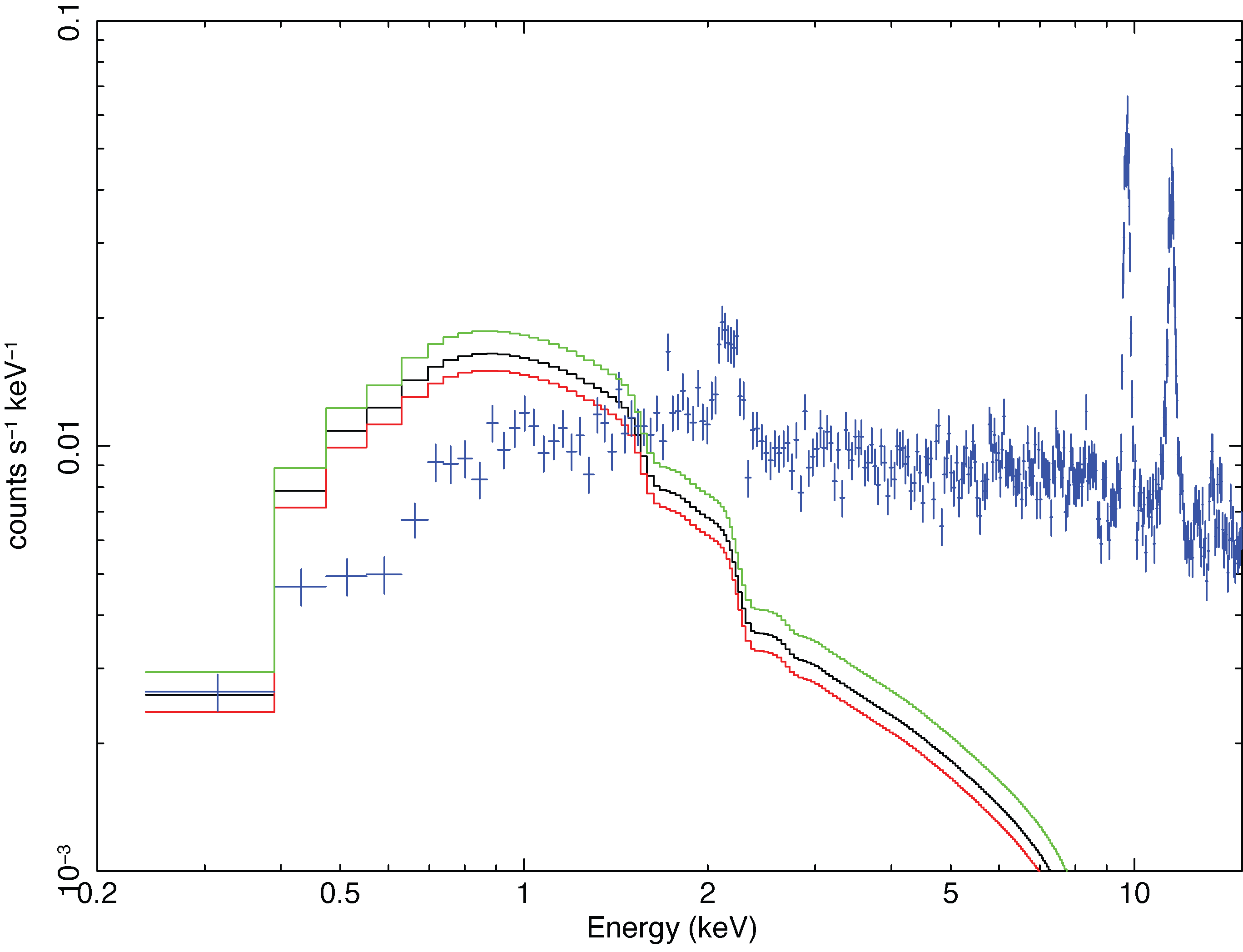 Example: Including Cosmic X-ray Background in a SimulationIf you need to evaluate the contribution of sky background, you can add sky background components to your simulation. The following provides instructions on including the CXB component in an extended source simulation. You can replace CXB with another background component, add more model components, or assume a point source by tweaking the commands. First, we define two source models, one for the primary target and one for CXB, as shown in the tables below. Here, we assume the target has a kT = 2 keV APEC spectrum and CXB suffers absorption by NH =5e21 cm-2. The CXB power-law normalization, 5.13345e-05, is for a 5' radius circular region assumed for the applied flat arf (xtd_extflatcircle.arf). We multiply the CXB model by 1.1 as CXB emission is extended beyond 5', and some emission outside of that is included in the spectrum. Here, we choose the source number 100 for CXB, but you can pick any positive integer but 1, which is already taken by the primary target. ========================================================================
Model src:apec<1> Source No.: 1 Active/On
Model Model Component Parameter Unit Value
par comp
1 1 apec kT keV 2.00000 +/- 0.0
2 1 apec Abundanc 1.00000 frozen
3 1 apec Redshift 0.0 frozen
4 1 apec norm 1.00000E-02 +/- 0.0
________________________________________________________________________
========================================================================
Model cxb_5:powerlaw<1>*TBabs<2>*constant<3> Source No.: 100 Active/On
Model Model Component Parameter Unit Value
par comp
1 1 powerlaw PhoIndex 1.29000 +/- 0.0
2 1 powerlaw norm 5.13345E-05 +/- 0.0
3 2 TBabs nH 10^22 0.500000 +/- 0.0
4 3 constant factor 1.10000 +/- 0.0
________________________________________________________________________
We then work on the spectral files. An Xspec log snippet below shows files loaded to Xspec for this simulation. Xspec needs to load a spectrum file to simulate multiple emission sources. Since we do not yet have any source spectrum, we use the NXB background file as a dummy source spectrum. We input the same file for background. The net count rate of zero may look strange, but no worry! The dummy data file does not do anything for the simulation. Next, we input rmf and arf files for each emission source. We use the same rmf (xtend_sim_v20201009.rmf) and arf (xtd_extflatcircle.arf) files for them as they are both extended sources. If you simulate a point source, change the arf file to xtd_pointsource.arf. 1 file 1 spectrum
Spectrum 1 Spectral Data File: xtend_sim_nxb_v20201009_r5arcmin.pha
Net count rate (cts/s) for Spectrum:1 6.939e-18 +/- 1.222e-03 (0.0 % total)
Assigned to Data Group 1 and Plot Group 1
Noticed Channels: 1-4096
Telescope: HITOMI Instrument: SXI Channel Type: PI
Exposure Time: 1.153e+05 sec
Using fit statistic: chi
Using Background File xtend_sim_nxb_v20201009_r5arcmin.pha[back]
Background Exposure Time: 1.153e+05 sec
Using Response (RMF) File xtend_sim_v20201009.rmf for Source 1
Using Auxiliary Response (ARF) File xtd_extflatcircle.arf
Using Response (RMF) File xtend_sim_v20201009.rmf for Source 100
Using Auxiliary Response (ARF) File xtd_extflatcircle.arf
Here are the actual commands for the above setup on Xspec. Although we explain from the source model, we need to load the data and response files first, or we get errors. We type the resp and arf commands twice for the primary source and CXB. The commands are the same except for the first number of the statements. We use 1 for the primary source and 100 for CXB. You can find a detailed explanation of the command syntax on the NICER SCORPEON page. data 1:1 xtend_sim_nxb_v20201009_r5arcmin.pha
back 1 xtend_sim_nxb_v20201009_r5arcmin.pha
response 1:1 xtend_sim_v20201009.rmf
arf 1:1 xtd_extflatcircle.arf
response 100:1 xtend_sim_v20201009.rmf
arf 100:1 xtd_extflatcircle.arf
model 1:src apec
2 0.01 0.008 0.008 64 64
1 -0.001 0 0 5 5
0 -0.01 -0.999 -0.999 10 10
0.01 0.01 0 0 1e+20 1e+24
model 100:cxb_5 powerlaw*TBabs*constant
1.29 -0.01 -3 -2 9 10
5.13345e-05 -0.01 0 0 1e+20 1e+24
0.5 -0.001 0 0 100000 1e+06
1.1 -0.01 0 0 1e+10 1e+10
Now, we can see the assumed spectrum model on an Xspec window. The bottom figure hides the data plots. 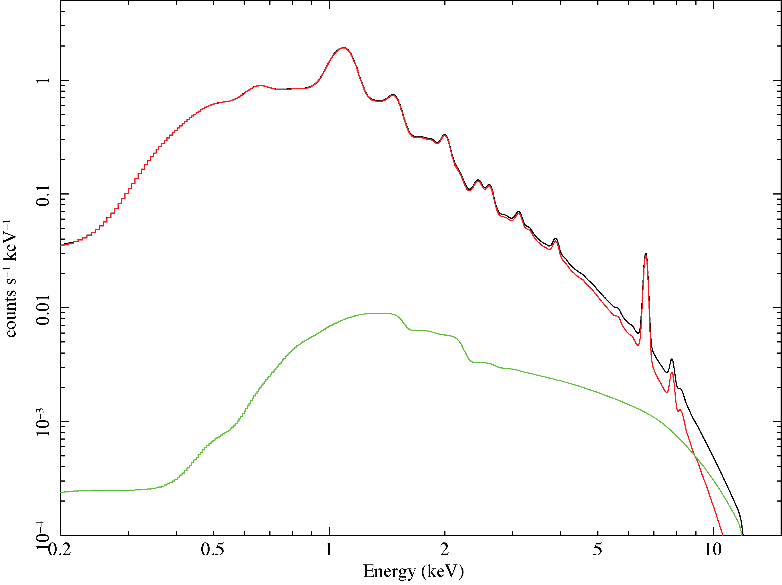 Finally, let's simulate a spectrum with the fakeit command on Xspec. Just type fakeit, then Xspec asks if we use counting statistics, so answer yes or hit return. We choose the filename, xtend_apec2keV_cxb_100ks.fak. Then, we input the exposure times for the source and background simulations, and here we simulate a 100 ksec exposure observation. As for the background exposure, we plan to use the NXB database, which the Xtend team will accumulate from night-earth observations. We have yet to know how much data are available, but we expect enough photon statistics for NXB, based on our experience with the the Suzaku mission. Here, we input 500 ksec for the background exposure. XSPEC12>fakeit
Use counting statistics in creating fake data? (y):
Input optional fake file prefix: xtend_apec2keV_cxb_100ks
Fake data file name (xtend_apec2keV_cxbxtend_sim_nxb_v20201009_r5arcmin.fak): xtend_apec2keV_cxb_100ks.fak
Exposure time, correction norm, bkg exposure time (115328., 1.00000, 115328.): 100000, 1.00000, 500000
Xspec outputs the following source and background spectral files. You can evaluate the error ranges with them. xtend_apec2keV_cxb_100ks.fak
xtend_apec2keV_cxb_100ks_bkg.fak

|

- HEASARC Director: Vacant
- NASA Official: Ryan Smallcomb
- Web Curator: J.D. Myers
- Last Modified: 2-Apr-2025