Resolve NXB Spectral Models
Resolve NXB spectral model version 3
Version 3 is the current version of the Resolve NXB spectral model, and should be used for analysis of XRISM Resolve spectra.
XSPEC model file
- xrism_nxb_v3_rsl_model.xcm
- This Resolve NXB model includes scale factors that permit easy scaling with the number of pixels. The scale factors were renormalized for Resolve NXB database v3 with CORTIME ≥ 6.
- Edit this file to specify the source number you want associated with this model.
M-size RMF
- xrism_nxb_v3_rsl_M.rmf
- This RMF is produced for the entire v3 NXB database, with the following filtering:
- When fitting data and model, do not apply the source RMF and ARF to the background model, but use this NXB-based RMF instead with no ARF. The full-database RMF likely suffices for most applications, but for sub-array analysis, we recommend making an RMF from the event file that is output by rslnxbgen. See Section 6.7 of the XRISM Data Analysis Guide for more information.
The model is based on characterization of the spectrum produced from an event file derived from the total NXB database v3, screened on EHK, including
CORTIME >= 6
and on event parameters according to:
(PI>=600) && ((RISE_TIME+0.00075*DERIV_MAX)>46) &&
((RISE_TIME+0.00075*DERIV_MAX)<58) && (ITYPE==0) &&
(STATUS[4]==b0) && (PIXEL!=27)
Thus, the model is presently based on 34 pixels and on Hp grade events only. NOTE: Even if any non-Ls grades (ITYPE < 4) were accepted, the result would be equivalent, as the file contains a negligible number of non-Hp grade events
The model was fitted from 1−17 keV using C statistics to data binned such that each bin has a minimum of one count.
Description of the model
- power-law + 25 Lorentzians + 5 scale factors that are described below under How to use the model
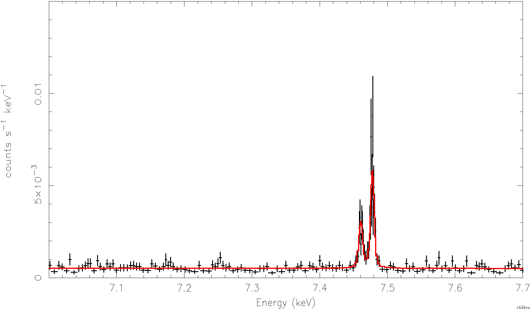
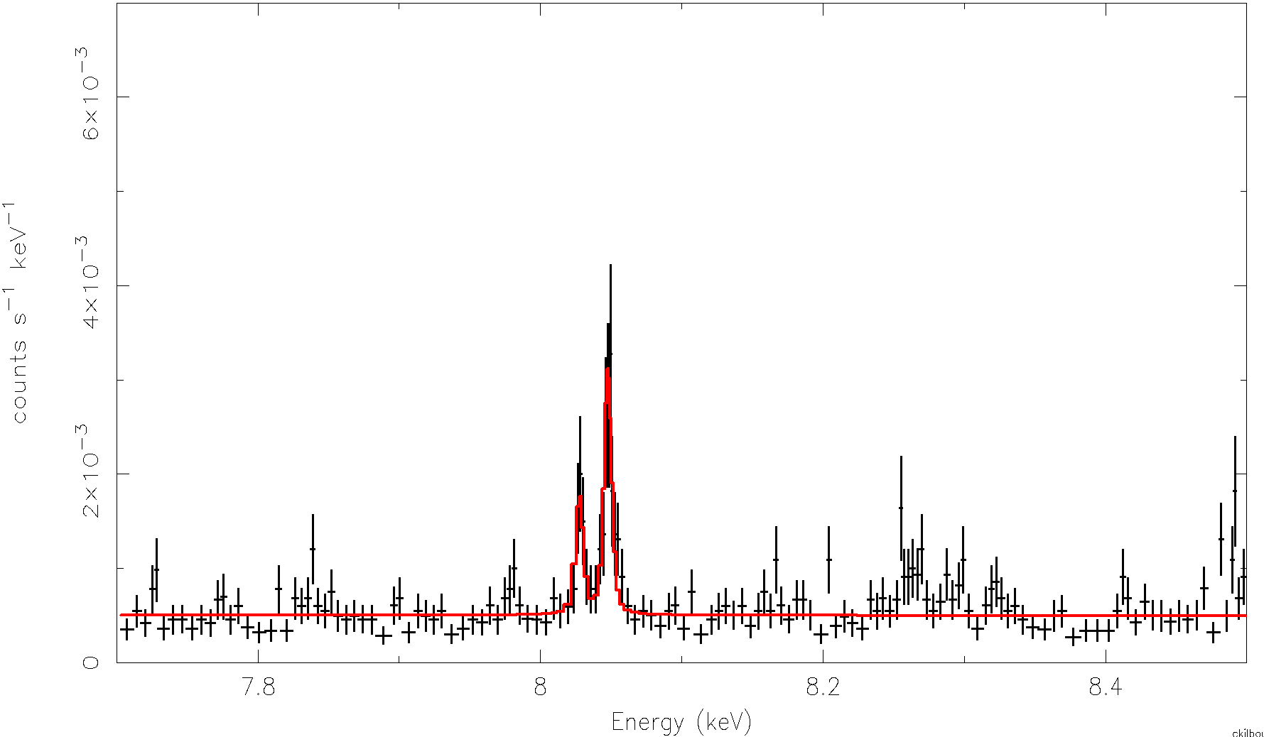
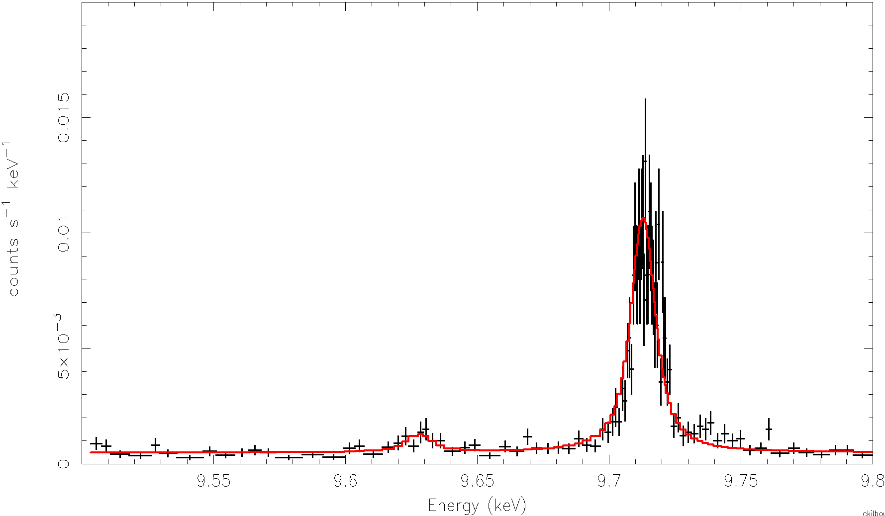
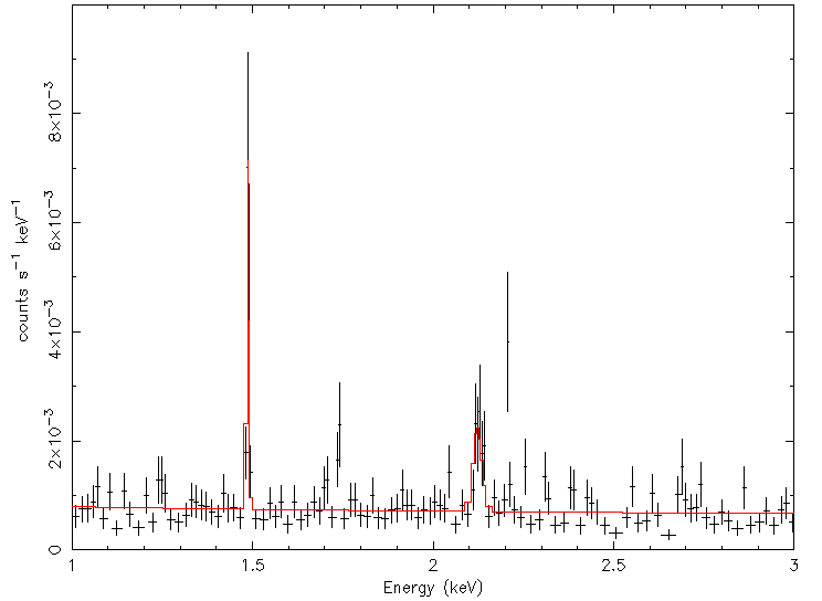
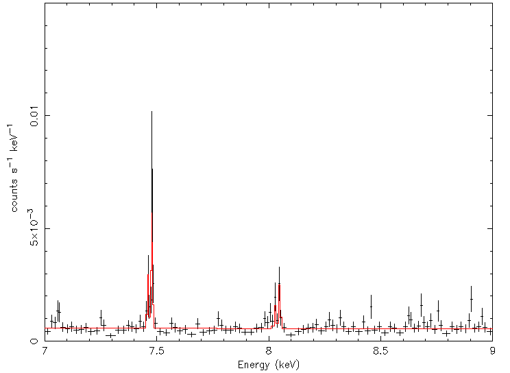
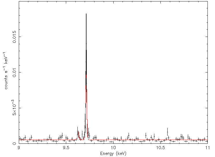
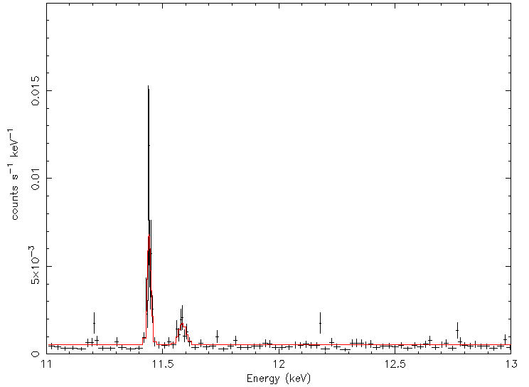
- Lines represented (number of Lorentzians used): Al-Ka (1), Si-Ka (1), Au-Ma (3), Au-Mb (3), Cr-Ka1/Ka2 (2), Mn-Ka1/Ka2 (2), Fe-Ka1/Ka2 (2), Ni-Ka1/Ka2 (2), Cu-Ka1/Ka2 (2), Au-La1 (1), Au-La2 (1), Au-Lb1 (1), Au-Lb2 (3), Au-Lg1 (1)
- Si Ka was omitted previously because it is a redistribution line included in all Resolve RMFs greater than size S. However, for weak sources, including the NXB component can reduce the residuals at that energy.
- Approximated Ka1/Ka2 lines by two Lorentzians instead of multiple Lorentzians needed to characterize the satellite lines
- We do not have the statistics to warrant complicating the model
- For Cr, Mn, Fe, Ni, and Cu lines, the Lorentzian width is frozen at the best fit value found in fits to the same lines in high-statistics, ground-calibration data, with the instrumental FWHM fixed at the value obtained from fitting the more detailed multi-Lorentzian model from Hölzer et al. 1997, Phys. Rev. A 56, 4554 to the line complex.
- Line intensity ratio of Ka1/Ka2 was not required to be 2:1
- Al and Si Ka were characterized as single Lorentzians since the doublet is not resolved.
- Shapes of the Au lines were determined empirically from high-statistics ground data accumulated specifically for this purpose. The model is valid for Hp grade events from 1−17 keV.
- The model is based on the premise that the spectrum (except for the Mn lines) is normalized by the cosmic ray rate but does not otherwise vary. The Mn lines should scale only according to the decay of Fe-55.
Characterizing the Au line shapes
- We used a calorimeter with slightly worse resolution than Resolve
- Au was a target in a rotating target source, so we obtained contemporaneous energy-scale calibration data and FWHM(E)
- Data when Au target was in place could be separately analyzed.
- Two day-long data sets were calibrated separately and merged.
- Models of lines (or line groupings) were tested on restricted-band NXB data before using them in the global model.
How to use the model
- The model contains 5 scale factors (parameters 1, 4, 11, 81, 82) and 15 independent normalization parameters (3, 7, 14, 20, 26, 32, 38, 41, 44, 53, 62, 65, 68, 74, 80). These may never all be free at the same time!
- Parameters 1 and 11 control the scaling of the continuum and all the lines except Mn. These should remain tied together.
- par 4 controls the scaling of the Mn lines. It would be redundant with par 7 except for the restricted fitting range set for par 7 (see discussion below).
- par 81 = 1/34 and should never be changed. It enables par 82, which should be set to the number of pixels used.
- We recommend using rslnxbgen to create an NXB spectrum weighted by the COR distribution of the observation you are analyzing and starting by fitting that before doing joint fits with the source data. Please refer to Resolve NXB Database and Spectral Extraction Recipes for more information.
- In the posted model file, all of the normalizations and scale factors are frozen except for parameter 1. The power-law index is also not frozen.
- All of the line energies and widths should be left frozen.
- The ranges for all of the parameter norms and the photon index have been constrained to ± 1-sigma from the fit used to determine these parameters.
- Even with a total exposure 3.66 Ms (after the CORTIME cut), the statistics in the Resolve NXB database result in error bars on the best-fit parameters that need to be considered when applying these parameters to individual observations.
- In order to account for this uncertainty, yet keep fits to the NXB in observations from producing unrealistic results, we recommend leaving the parameter ranges at the ± 1-sigma values provided in the posted model.
- When fitting, check whether any parameter has reached a limit of its allowed range and adjust the range as needed.
- First fit the model with all of the normalizations and scale factors frozen except for par 1.
- If you are using fewer than 34 pixels, first change par 82 to the actual number of pixels involved
- This will allow the normalizations of the model to start out closer to the correct values.
- The power-law index (par 2) is also intended to be left free during this and the subsequent step, with the range constrained as specified in the model file.
- Fitting for par 1 is done to adjust the common scale of the particle-induced background.
- We do not expect that par 1 will need to vary much, as we expect the COR distribution within most individual observations to be similar to each other and to the NXBDB.
- We also do not expect par 2 to change much.
- The distribution of scattered cal-source photons across the array is non-uniform; thus, for sub-array groups, par 4 must be allowed to vary separately
- Next freeze par 1 (and par 4 if it was thawed), thaw parameters 3, 7, 14, 20, 26, 32, 38, 41, 44, 53, 62, 65, 68, 74, 80, and fit again.
- This is done to allow adjustment to the normalization of the individual parameters within the allowed ± 1-sigma range.
Example XSPEC commands
data rsl_nxb.pi   (replace with the NXB spectrum you generated for your observation)

response xrism_nxb_v3_rsl_M.rmf  (replace with the M-size RMF you generated from the event file produced by rslnxbgen if not analyzing the full array)

@xrism_nxb_v3_rsl_model.xcm

ignore 0.0-1.0, 17.0-99.0  (can choose a smaller range within 1 - 17 keV, of course)

(if needed) new 82 N   (where N is the number of pixels being used)

(if needed) thaw 4

fit

freeze 1

(if thawed) freeze 4

thaw 3, 7, 14, 20, 26, 32, 38, 41, 44, 53, 62, 65, 68, 74, 80

fit  (check whether any parameters are at the limits of their fit ranges and adjust)
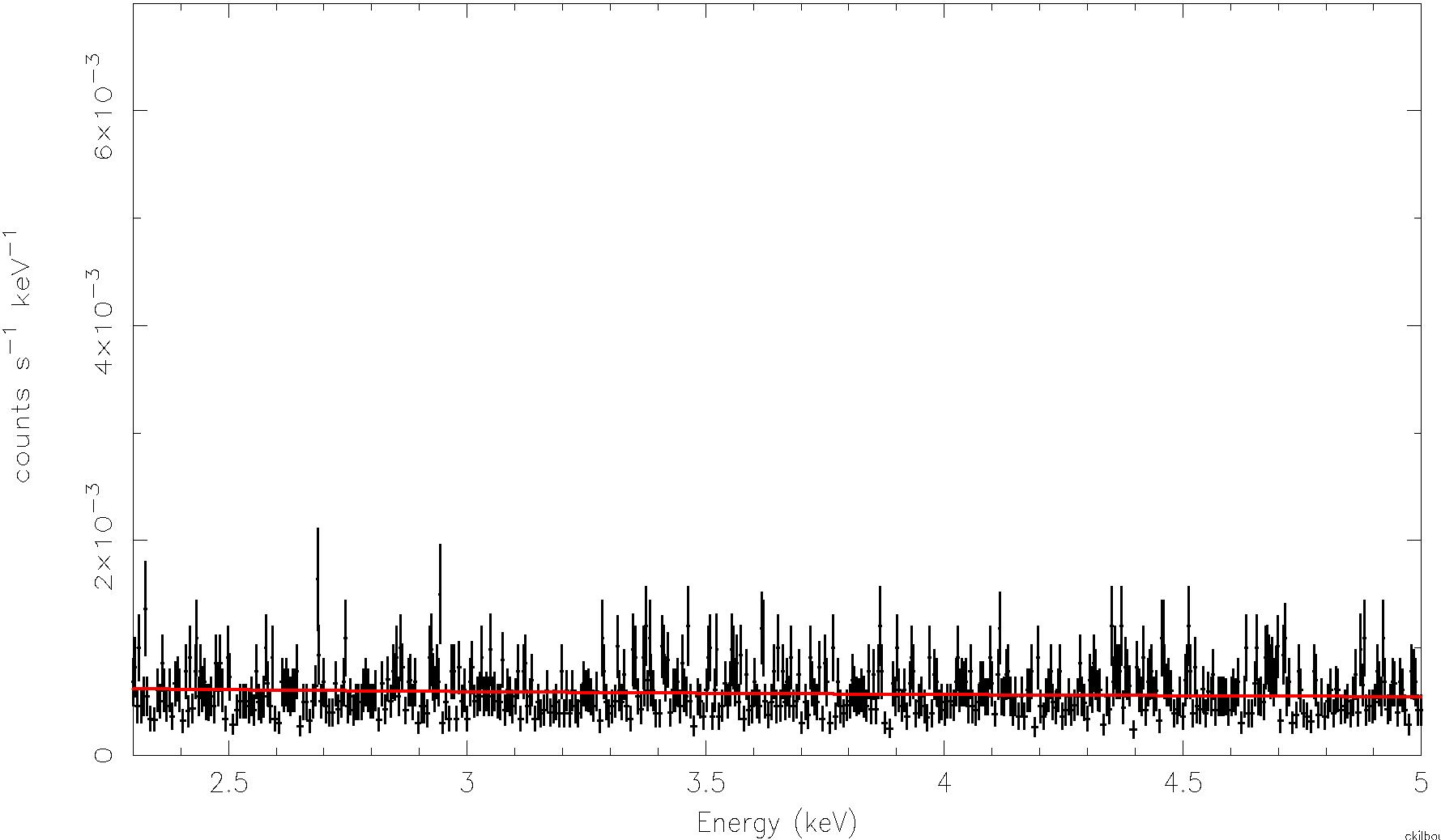
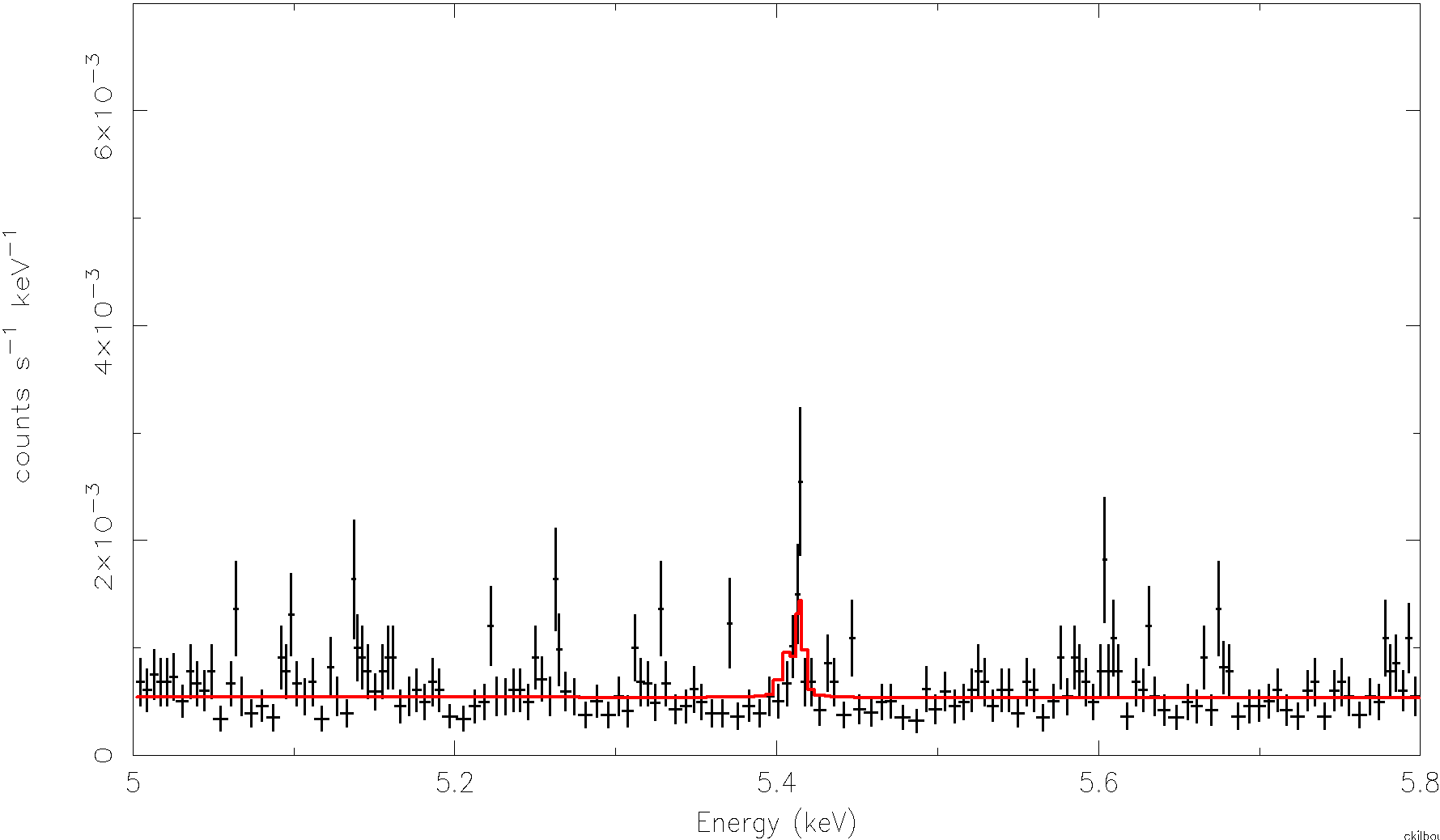
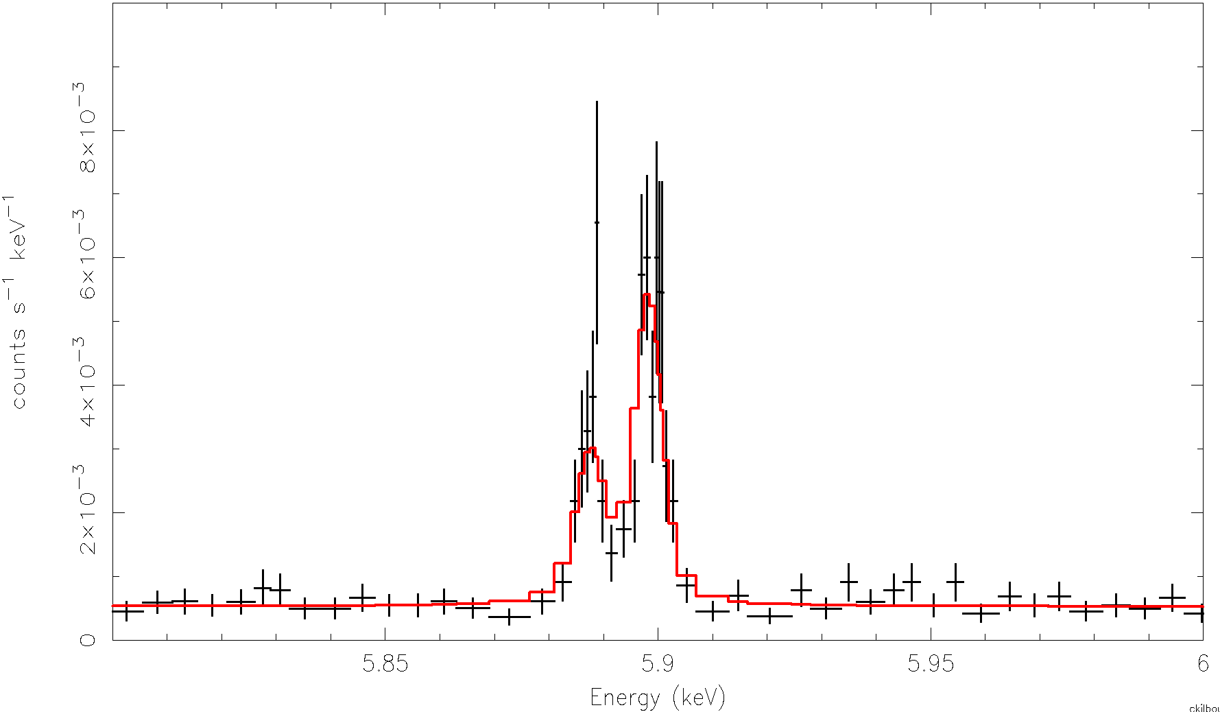
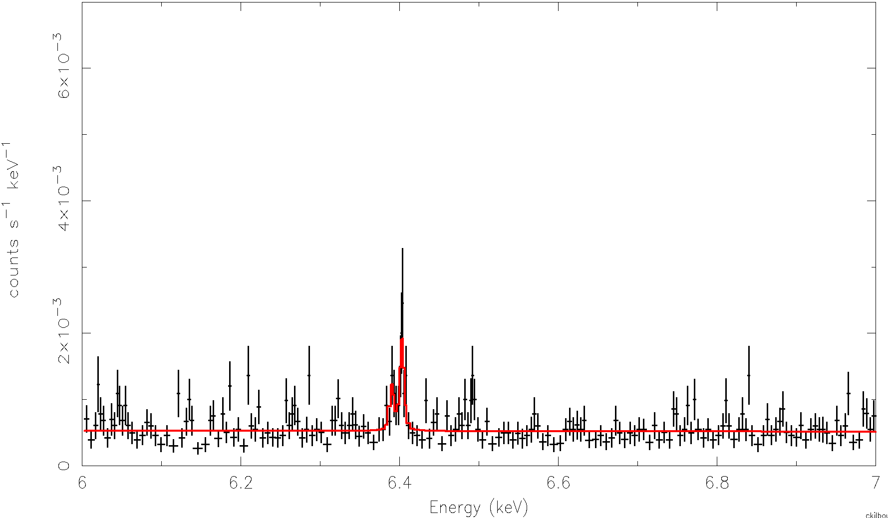
Spectra with the model overlaid
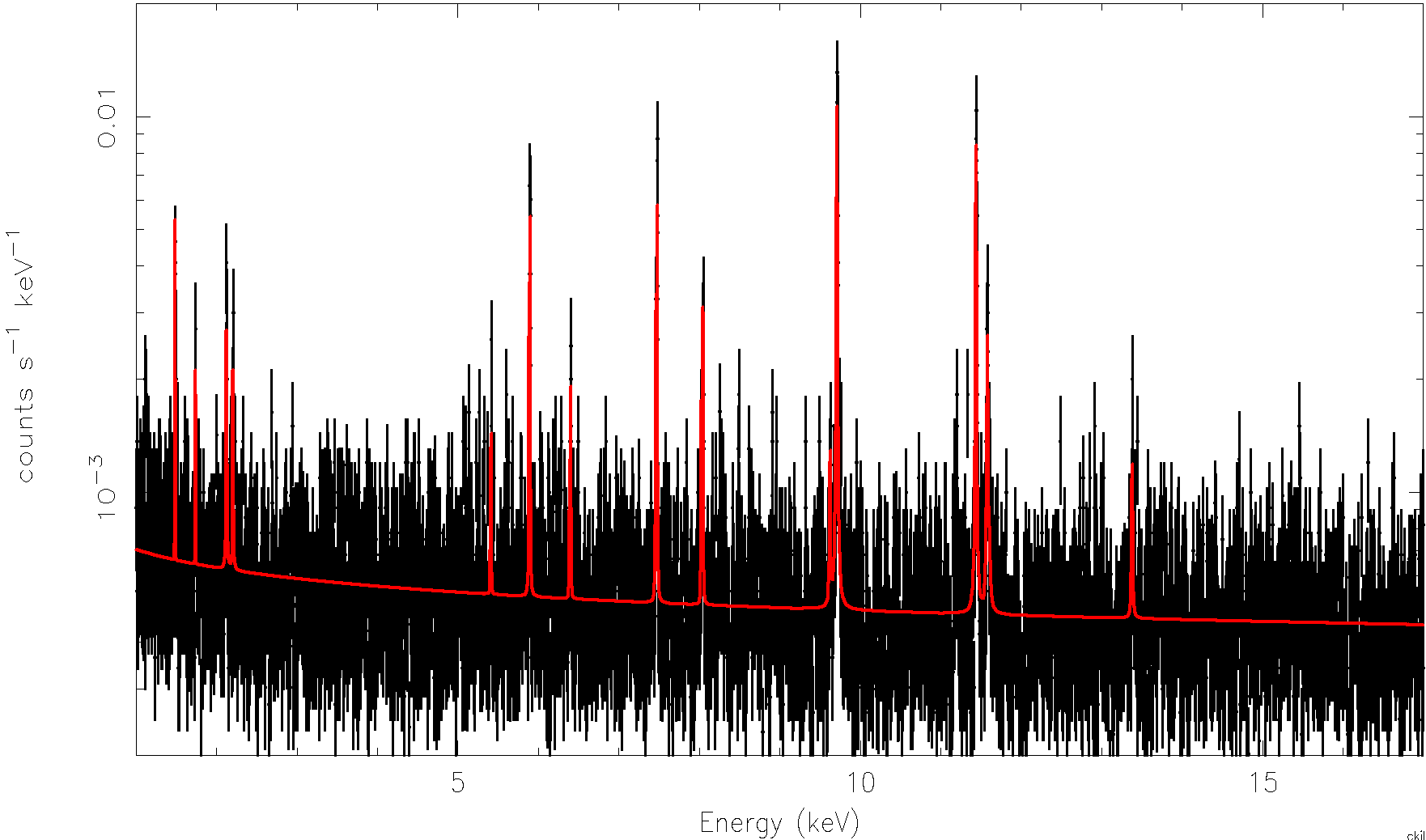
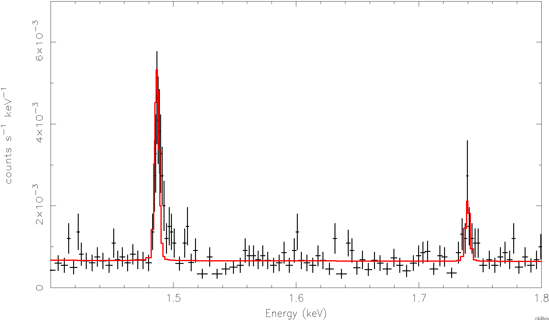
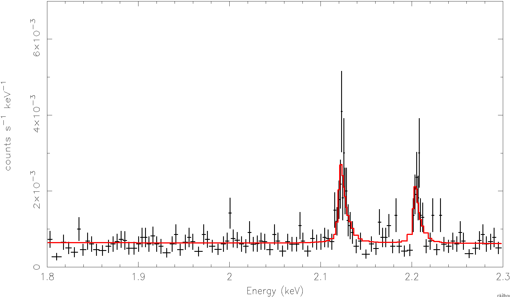
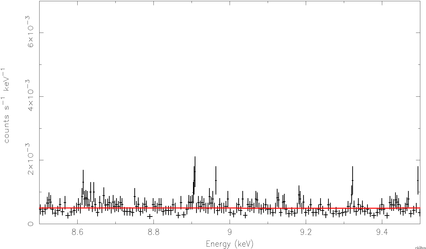
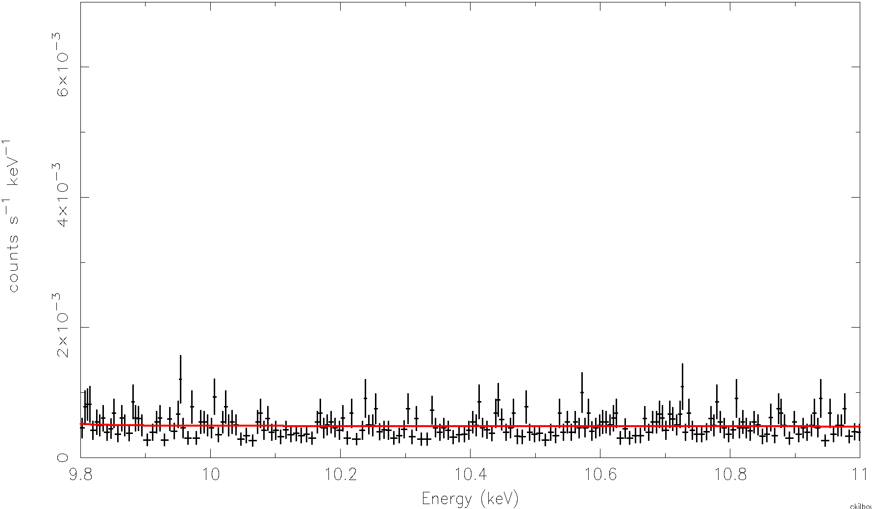
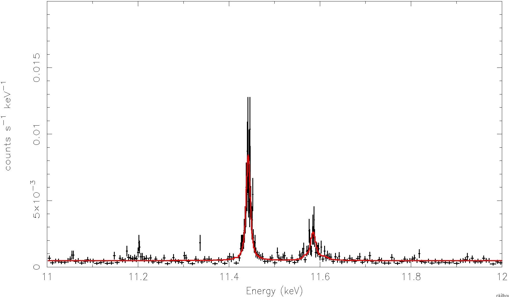
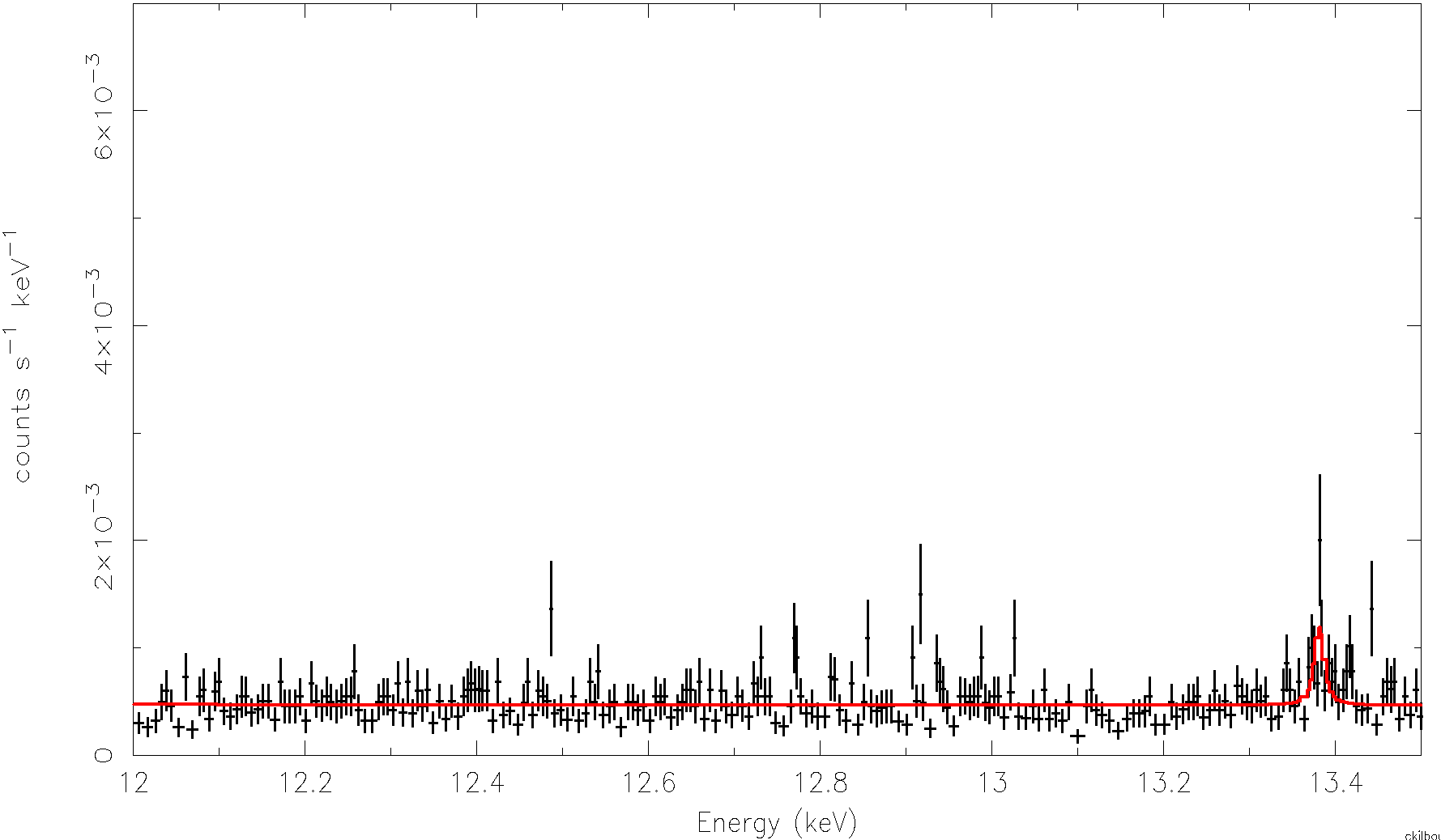
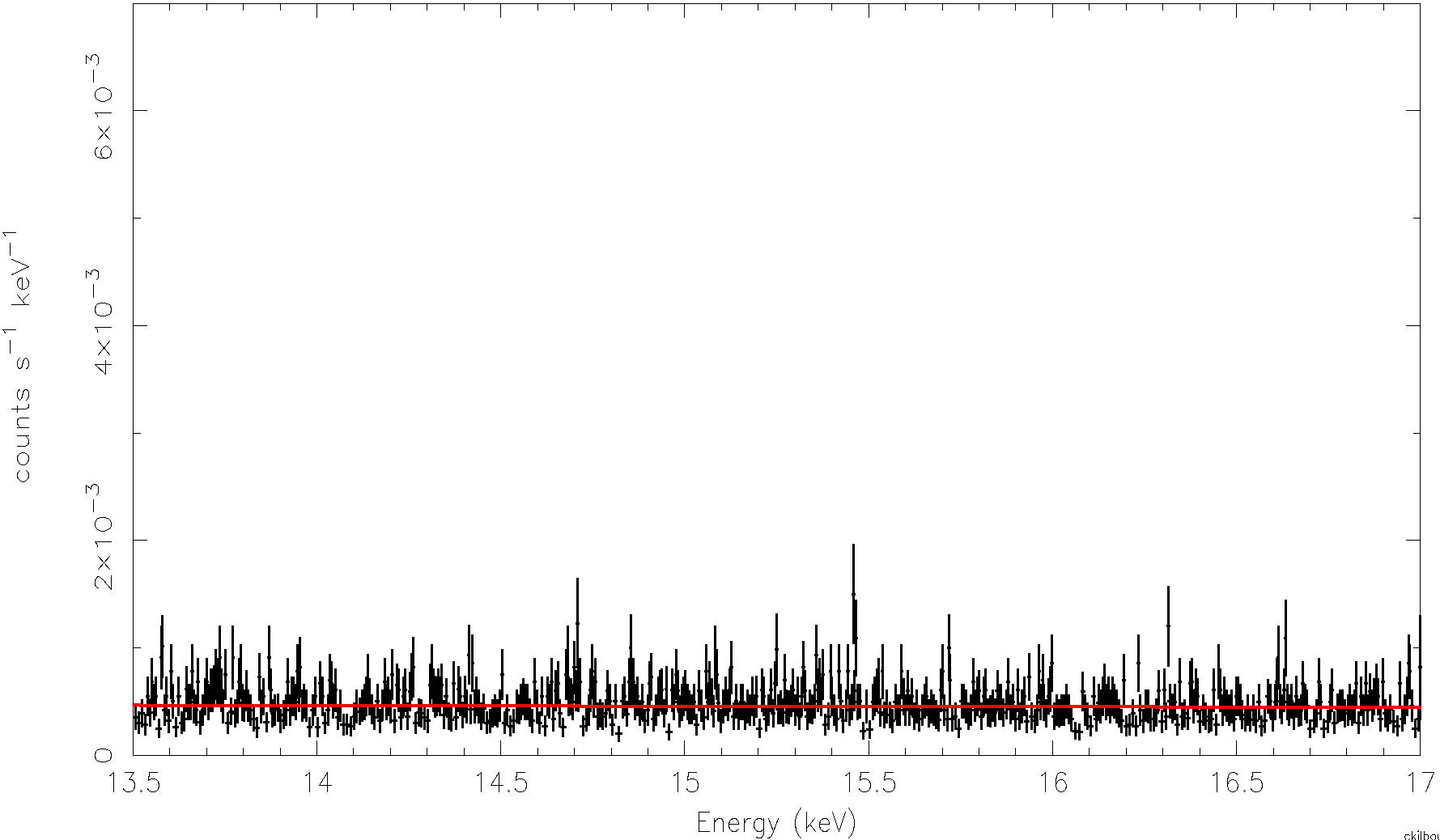
Note that the binning shown is for visualization and is not what was used for the fitting. Because adaptive binning was used for these plots (setplot rebin 3 10), positive fluctuations will tend to get isolated in smaller bins while negative fluctuations will get averaged out. This effect is likely why the lines tend to have spikes that exceed the model.
Limitations of the model and likely future improvements
- The model cannot account for transient changes in background, such as from unusual solar activity.
- Please continue to report unusual line energies or intensities.
- Consider the uncertainties when applying the full array model to a small subset of pixels.
Resolve NXB spectral model version 2
Version 2 of the Resolve NXB model is deprecated, please use the most recent version at the top of this page. This material is retained for reference.
Version 2 of the Resolve NXB spectral model updates the descriptions of the Au lines and adds several new lines. More fundamentally, it no longer includes the instrumental broadening in the model, but relies on creation of an RMF (M-size). This approach was taken so that the lines could be specified as Lorentzians rather than Voigts, which was motivated in part by the use of a different calorimeter with somewhat worse spectral resolution than Resolve to obtain the Au fluorescence spectra that were used to determine the Au line shapes.
XSPEC model file
- xrism_nxb_v2_rsl_model.xcm
- New Resolve NXB model with scale factors that permit easy scaling with number of pixels
- Edit this file to specify the source number you want associated with this model.
M-size RMF
- xrism_nxb_v2_rsl_M.rmf
- This RMF is produced for the entire v2 NXB database.
- When fitting data and model, do not apply the source RMF and ARF to the background model, but use this NXB-based RMF instead with no ARF. The full-database RMF likely suffices for most applications, but for sub-array analysis, we recommend making an RMF from the event file that is output by rslnxbgen.
The model is based on characterization of the spectrum produced from an event file derived from the total NXB database V2, screened on EHK, and screened further on event parameters according to:
(PI>=600) && ((RISE_TIME+0.00075*DERIV_MAX)>46) &&
((RISE_TIME+0.00075*DERIV_MAX)<58) && (ITYPE==0) &&
(STATUS[4]==b0) && (PIXEL!=27)
Thus, the model is presently based on 34 pixels and on Hp grade events only. NOTE: Even if any non-Ls grades (ITYPE < 4) were accepted, the result would be equivalent, as the file contains a negligible number of non-Hp grade events.
Description of the model
- power-law + 25 Lorentzians + 5 scale factors that are described below under How to use the model
- New lines represented (number of Lorentzians used): Al-Ka (1), Si-Ka (1), Au-Ma (3), Au-Mb (3), Cr-Ka1/Ka2 (2), Mn-Ka1/Ka2 (2), Fe-Ka1/Ka2 (2), Ni-Ka1/Ka2 (2), Cu-Ka1/Ka2 (2), Au-La1 (1), Au-La2 (1), Au-Lb1 (1), Au-Lb2 (3), Au-Lg1 (1)
- Si Ka was omitted previously because it is a redistribution line included in all Resolve RMFs greater than size S. However, for weak sources, including the NXB component can reduce the residuals at that energy.
- Approximated Ka1/Ka2 lines by two Lorentzians instead of multiple Lorentzians needed to characterize the satellite lines
- We do not have the statistics to warrant complicating the model
- For Cr, Mn, Fe, Ni, and Cu lines, the Lorentzian width is frozen at the best fit value found in fits to the same lines in high-statistics, ground-calibration data, with the instrumental FWHM fixed at the value obtained from fitting the more detailed multi-Lorentzian model from Hölzer et al. 1997, Phys. Rev. A 56, 4554 to the line complex.
- Line intensity ratio of Ka1/Ka2 was not required to be 2:1
- Al and Si Ka were characterized as single Lorentzians since the doublet is not resolved.
- Shapes of the Au lines were determined empirically from high-statistics ground data accumulated specifically for this purpose
- The model is valid for Hp grade events from 1−17 keV.
- The model is based on the premise that the spectrum (except for the Mn lines) is normalized by the cosmic ray rate but does not otherwise vary. The Mn lines should scale only according to the decay of Fe-55.
Characterizing the Au line shapes
- We used a calorimeter with slightly worse resolution than Resolve
- Au was a target in a rotating target source, so we obtained contemporaneous energy-scale calibration data and FWHM(E)
- Data when Au target was in place could be separately analyzed.
- Two day-long data sets were calibrated separately and merged.
- Models of lines (or line groupings) were tested on restricted-band NXB data before using them in the global model.
How to use the model
- The model contains 5 scale factors (p1, 4, 11, 81, 82) and 15 independent normalization parameters (p3, 7, 14, 20, 26, 32, 38, 41, 44, 53, 62, 65, 68, 74, 80). These may never all be free at the same time!
- Parameters 1 and 11 control the scaling of the continuum and all the lines except Mn. These should remain tied together.
- p4 controls the scaling of the Mn lines. It would be redundant with p7 except for the restricted fitting range set for p7 (see discussion below).
- We recommend using rslnxbgen to create an NXB spectrum weighted by the COR distribution of the observation you are analyzing and starting by fitting that before doing joint fits with the source data.
- In the posted model file, all of the normalizations and scale factors are frozen except for parameter 1.
- All of the line energies and widths should be left frozen.
- The ranges for all of the parameter norms and the photon index have been constrained to ± 1-sigma from the fit used to determine these parameters.
- Even with a total exposure of 2.67 Ms, the statistics in the Resolve NXB database result in error bars on the best-fit parameters that need to be considered when applying these parameters to individual observations.
- In order to account for this uncertainty, yet keep fits to the NXB in observations from producing unrealistic results, we recommend leaving the parameter ranges at the ± 1-sigma values provided in the posted model.
- When fitting, check whether any parameter has reached a limit of its allowed range and adjust the range as needed.
- First fit the model with all of the normalizations and scale factors frozen except for p1.
- If you are using fewer than 34 pixels, first change p82 to the actual number of pixels involved
- This will allow the normalizations of the model to start out closer to the correct values.
- The photon index is also intended to be left free during this and the subsequent step, with the range constrained as specified in the model file.
- Fitting for p1 is done to adjust the common scale of the particle-induced background.
- We do not expect that p1 will need to vary much, as we expect the COR distribution within most individual observations to be similar to each other and to the NXBDB.
- The distribution of scattered cal-source photons across the array is non-uniform; thus, for sub-array groups, p4 must be allowed to vary separately
- Please consult v2 files, spatial distribution, and spectrum for the v2 uniformity maps.
- Next freeze p1 (and p4 if it was thawed), thaw p3, 7, 14, 20, 26, 32, 38, 41, 44, 53, 62, 65, 68, 74, 80, and fit again.
This is done to allow adjustment to the normalization of the individual parameters within the allowed ± 1-sigma range.
Limitations of the model and likely future improvements
- The model cannot account for transient changes in background, such as from unusual solar activity.
- Please continue to report unusual line energies or intensities.
- Consider the uncertainties when applying the full array model to a small subset of pixels.
Resolve NXB spectral model version 1
Version 1 of the Resolve NXB model is deprecated, please use the most recent version at the top of this page.
rsl_nxb_model_v1.mo (first released empirical background model, nxb1)
newdiag60000.rmf (unity diagonal matrix for use with background model)
When fitting data and model, don't apply the source RMF and ARF to this background model, but use the diagonal RMF instead and no ARF. The model will be entered as model 2.
data 1:1 <data>
resp 1:1 <rmf>
arf 1:1 <arf>
resp 2:1 newdiag60000.rmf
The model is based on characterization of the spectrum produced from an event file derived from the total working preliminary NXB database, screened on EHK as described on the Resolve NXBDB page, and screened further on event parameters according to:
(PI>=600) && ((RISE_TIME+0.00075*DERIV_MAX)>46) && ((RISE_TIME+0.00075*DERIV_MAX)<58) && (ITYPE==0) && (STATUS[4]==b0) && (PIXEL!=27)
Note then that the model is presently based on 34 pixels and on H events only.
Description of the model
- The model is empirical and is intended simply to describe the background we measure, and not some fundamental spectrum that is altered by the instrument response.
- Because of this, the instrumental broadening of the lines is included in the model.
- power-law + 17 Gaussians + 3 scale factors that will be described in "How to use the model"
- Lines represented: Al-Ka1/Ka2, Au-Ma1, Cr-Ka1/Ka2, Mn-Ka1/Ka2, Fe-Ka1/Ka2, Ni-Ka1/Ka2, Cu Ka1/Ka2, Au-La1/La2, Au-Lb1/Lb2
- The lines are approximated as Gaussians although each line is really made up of multiple Lorentzians, each broadened by the LSF.
- This approximation was chosen because the statistics of the background do not justify specifying the known detailed descriptions of each line complex.
- For the Al, Cr, Mn, Fe, Ni, and Cu lines, we fixed the sigma parameter of the Gaussians at values consistent with fits of Gaussians to the same lines in high-statistics, ground-calibration data.
- The shapes of the Au lines were not available in the literature, thus they are entirely described by the fits to the background data file.
- Si-Ka1/Ka2 are not included in the model because these lines are also produced as part of the spectral redistribution of observed sources, which usually dominates. This redistribution is included in the XL RMF.
- Central energies of the lines are fixed to the values in https://xdb.lbl.gov/Section1/Table_1-3.pdf. (X-RAY DATA BOOKLET, Center for X-ray Optics and Advanced Light Source, Lawrence Berkeley National Laboratory)
- Sigmas of Gaussian models of Ka1 and Ka2 lines for each element are tied and fixed.
- Line intensity ratio of Ka1 to Ka2 is set to be 2:1 for each element.
- The model is valid for H events from 1 - 17 keV.
- The model is based on the premise that the spectrum (except for the Mn lines) is normalized by the cosmic ray rate but does not otherwise vary. The Mn lines should scale only according the the decay of Fe-55.
Pictorial overview of the Resolve NXB and current model




How to use the model
- The model contains 3 scale factors (nxb1:1, 4, 11) and 12 independent normalization parameters (nxb1:3, 7, 14, 20, 23, 29, 35, 41, 47, 50, 53, 56). These may never all be free at the same time!
- Parameters 1 and 11 control the scaling of the continuum and all the lines except Mn. These should remain tied together.
- nxb1:4 controls the scaling of the Mn lines. It would be redundant with nxb1:7 except for the restricted fitting range set for nxb1:7 (see discussion below).
- We recommend using rslnxbgen to create an NXB spectrum weighted by the COR distribution of the observation you are analyzing and starting by fitting that before doing joint fits with the source data.
- In the posted model file, all of the normalizations and scale factors are frozen except for parameter 1.
- All of the line energies are frozen and should be left frozen.
- The ranges for all of the parameter norms, the photon index, and the widths of the Au lines have been constrained to +/- 1-sigma from the fit used to determine these parameters.
- Even with a total exposure of 785 ks, the statistics in the Resolve NXB database result in error bars on the best-fit parameters that need to be considered when applying these parameters to individual observations.
- In order to account for this uncertainty, yet keep fits to the NXB in observations from producing unrealistic results, we recommend leaving the parameter ranges at the +/- 1-sigma values provided in the posted model.
- First fit the model as delivered, with all of the normalizations and scale factors frozen except for parameter 1.
- Note that the photon index and the widths of the Au lines are intended to be left free during this and the subsequent step, with the ranges constrained as specified in the model file.
- This is done to adjust the common scale of the particle-induced background.
- We do not expect that parameter 1 will need to vary much, as we expect the COR distribution within most individual observations to be similar to each other and to the NXBDB.
- To set an extreme example, we divided the NXBDB into two parts, COR < 10.67 and ≥ 10.67.
- The new best-fit values for nxb1:1 were 1.21 and 0.832, respectively. No real observation would have a COR distribution as extreme as these contrived COR mixes.
- Of course, if you are analyzing fewer than 34 pixels, nxb1:1 will need adjustment, accordingly.
- The distribution of scattered cal-source photons across the array is non-uniform, so for spectra using fewer than 34 pixels, scaling nxb1:4 by number of pixels is not appropriate; see below. Of the 64 counts between 5.88 - 5.91 keV, 8 of them are in Pixel 11, and 6 in Pixel 15.
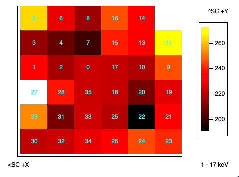
- Note that the full 1 - 17 keV distribution across the array could also be somewhat non-uniform. The mean number of counts per pixel is 227.92, and the standard deviation is 16.65, whereas 15.10 would be expected for sqrt(mean).
- Next freeze nxb1:1, thaw nxb1:3, 7, 14, 20, 23, 29, 35, 41, 47, 50, 53, 56, and fit again.
- This is done to allow adjustment to the normalization of the individual parameters within the allowed +/- 1-sigma range
Limitations of the model and likely future improvements
- The shapes of the Au lines are currently not constrained by anything other than the fit to the integrated NXB. Resolve team members at LLNL are taking measurements now to help provide better constraints for these lines.
- We may also add Au Mb and Lg.
- There are suggestions of other lines in the data, but we did not have the statistics to constrain their normalizations. They must affect the description of the continuum to some extent.
- If the use of the Gaussian approximation causes problems in the fitting, the next step would be to use Voigt profiles constrained by fits to the ground data.
- There is a weak indication that the shape of the spectrum, in addition to the scaling, depends on COR.
- We compared the ratio of counts 12 - 17 keV / 1 - 12 keV for COR < 10.67 and ≥ 10.67 in the NXBDB.
- LOW COR hardness ratio = 0.34 +/- 0.01 (assuming sqrt(N) errors)
- HIGH COR hardness ratio = 0.36 +/- 0.01 (assuming sqrt(N) errors)
- This difference was also reflected in the spectral index and normalizations obtained for the power laws of the two parts, though in both cases the new results were (barely) within 1-sigma of the fit to the full data set.
- We expect that, since the effect is marginal when dividing the data into low and high COR values, variations in the COR distributions of typical data sets will correspond to negligible spectral variation.
- We look forward to increasing the statistics in the NXBDB so that we can characterize potential spectral changes.
- The model cannot account for transient changes in background, such as from unusual solar activity.
- Please continue to report unusual line energies or intensities.
- Consider the uncertainties when applying the full array model to a small subset of pixels.
|