National Aeronautics and Space Administration

THE EXOSAT SUM SIGNAL EFFICIENCY CORRECTION :
DIRECT COMPUTATION FROM THE DATA

Readers not familiar with the CMA sum signal and its usage to compute the sum signal-dependent efficiency correction are referred to the FOT Handbook, section 8.1.3 for an introduction. The basic facts are summarised below, then a new method (not described in the FOT Handbook) to compute the efficiency correction directly from the data, without the use of the CCF, is presented.

The sum signal is the summed output from the readout contacts on the CMA resistive disc. It appears as an ADC channel number (0-127) for each event in the IM packet. Since only events with a signal above a given threshold (PET=Position Encoding Threshold) on any of the four contacts are considered valid, a sum signal histogram (counts vs ADC channel no.) will start abruptly at a given ADC channel, which is a function of the PET setting (so far con- stant) and of the position in the field of view.

Events in channel O and 1 are spurious and should be disregarded. Since the CMA efficiency given in the CCF was calculated using no PET, a correction is necessary for a sum signal-dependent factor. This is simply the ratio between the area of the sum signal distribution above the threshold, and the total area (with no threshold). This method was used to generate the correction factors in the CCF from the ground measurements (monochromatic X-rays).

Data analysis at the EXOSAT Observatory has shown that the values in the CCF are only guidelines to the in-flight behaviour (cosmic sources are not monochromatic!). In particular, for a given sum signal distribution and its median, the correction factor obtained from the CCF is underestimated in comparison to the directly computed value.This implies that a larger correction is necessary, i.e. the actual correction coefficient (which is a number between O and 1) is lower (further from 1) than the predicted value.

The difference is small for most of the normal X-ray distributions (for which the correction factor is in any case close to 1), but could be non-negligible for softer distributions (lower sum signal median).

The following method may be used to compute the efficiency correction directly from the data. It assumes that a Pearson type I distribution describes the source sum signal distribution; this is confirmed in practice. Naturally, the parameters of the Pearson distribution are different from those for a monochromatic distribution. No attempt has been made to model the sum signal distribution from a continuum as a convolution of monochromatic distributions: the Pearson fit provides a good empirical description.

1. Accumulate a signal histogram y=f(x) using a set of values y_i for each channel i=0,127. The associated sum signal value may be derived as x_i=i-0.5.
2. Locate the threshold to define the first channel to be fitted. This can be done very easily by eye, or an automatic algorithm may be developed.
3. Fit the data with the modified Pearson type I distribution

y = K ( 1 + (x - x0) / a1 )m1 . (1 - (x - x0) / a2)m2

where the five parameters K, x₀, a₁, m₁, m₂ are variable and the following relation holds m₁/a₁ = m₂/a₂. A least squares fit method (e.g. Bevington's CURFIT) can be used.

4. The following assumptions are valid as initial parameter values:

K = height of the-peak of the distribution 
xO= channel of the peak of the distribution
a1= xO 
m1=ratio between the first channel (from the top) 
   with at least 10% of the peak counts, and xO 
m2= m1

The above guesses generally lead to a quick convergence. In a few specific cases the values require some adjustment (generally try to raise m₁ and m₂, i.e. make the distribution narrower). To select the initial parameters by eye, please note:

K controls the peak height, 
x0 and a1 control the peak position, 
m1 and m2 control the skewness of the left and right wing of the distribution.

5. Once the above parameters are calculated, the threshold for integration should be determined.

One possible method is to calculate the channel numbers corresponding to 80% and 20% of the histogram value at the threshold used for the fit (point 2 above). The values may be determined in fractional channel numbers using the y values for two adjacent channels (one above and one below 80% or 20%), the x values defined according to the convention at point 1 above, with a linear extrapolation. Further linear extrapolation can be used to derive a fractional channel number (corresponding to 50% of the initial y value at the threshold), which is the integration threshold.

6. Integrals of the fit on all the channels and on that part above the threshold determined at point 5 are computed. A straightforward numeric integration (histogram summation) is sufficient.
7. The efficiency correction is the ratio of the two integrations.

The above is used by the program EFCOR in the EXOSAT Observatory LE Interactive Analysis System.

L. CHIAPPETTI

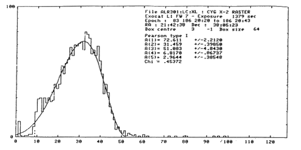
The top frame shows a sum signal histogram (and its Pearson fit) for a hard X-ray source (Cyg X-2). The integration threshold is at channel 9.0, and the efficency correction 97.4% ( compared with a CCF value of 98.8% obtained from the sum signal median value of 30.5).

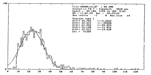
The bottom frame refers to a softer source (AN UMa). The integration threshold is at channel 8.4 and the efficency correction is 92.7% ( to be compared with a prediction of 97.4% using the sum signal median of 25.0).