GSPC CALIBRATIONS
Introduction
The first observation of the Crab made in 1983 with the GSPC on EXOSAT indicated
that the response of the detector as given by the pre-launch calculations and
calibrations was incorrect. A large deficiency in counts below 4 keV was apparent
along with a line feature in the spectrum around 4.78 keV. Effective areas as a
function of energy were modified to give the correct fit to the Crab. In addition
to these problems the absolute gain calibration as defined by two line features
in the background, which had been ascribed to Lead L fluorescence, did not give
the correct energy for the Sulphur line measured from Cas A. This suggested that
these lines might not be Lead, but rather were from Bismuth, perhaps caused by
the radio-active decay of a lead isotope.
Over the past few months a major effort has been made to obtain' a fuller
understanding of the GSPC response. This has, in part, been helped by the
performance of a long observation of the Crab made with the burst length
discriminator set to give a maximum acceptance range. This
discriminator is used to reduce the particle background, but also
removes a small percentage of X-rays in an energy dependent way. Since
the energy dependence of this process requires calibration, such an
observation was essential in order to investigate the above
problems. The appropriate observation of the Crab was made in February 1985.
Using data from this observation, considerable
progress has been made. A number of uncertainties in critical detector
parameters have come to light and make it possible to reproduce the
Crab spectrum to within 2% without making arbitrary changes to the
response. The following describes the various steps that were taken to
resolve the problem of the GSPC calibration.
It should be stressed that calibration of the GSPC, a
new instrument with a resolution approximately a factor of two better than that
of a conventional proportional counter, presented new and unexpected problems.
The improved resolution revealed many subtle effects that hitherto would have
gone unnoticed in a proportional counter. In retrospect, the ground
calibration fell short of what was required to fully model the nuances of the
instrument response.
1. The Absolute Energy Calibration
A
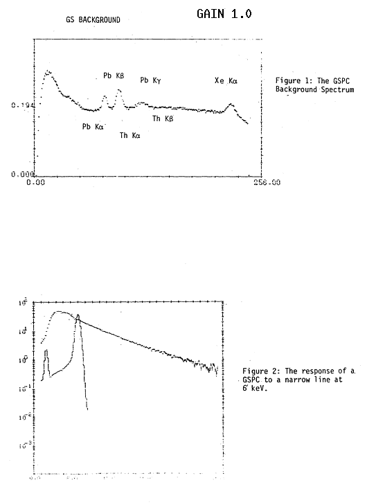
detailed study of the background spectrum has been made by P. de Korte. A
spectrum taken in gain one is shown in Figure I. This reveals a number of line
features that can be identified as resulting from three separate processes. First
the two strong lines between channels 65 and 100 are the L alpha and beta lines
from the fluorescence of lead in the collimator. A cursory glance at Figure 1
reveals that the L beta line is stronger than the alpha line, which is contrary
to the expected branching ratio of 110:70. This is caused by a second line
complex that overlaps the lead lines. The broad bump around channel 125 is a
blend of the lead L gamma line and a Thorium L beta line at 16.2 keV, the latter
resulting from the radioactive decay of residual plutonium in the Beryllium
window. The K alpha Thorium line is at 12.9 keV and lies very close to the lead K
beta line at 12.6 keV such that the upper of the two lead lines is a blend, which
can be treated as a single line with a mean energy of 12.703 keV. The energy of
the lead L alpha line is 10.541 keV.
The remaining line in the spectrum between channels 200
and 225 is identified with Xenon K alpha and arises from the escape photons of
high energy background particle events that are captured by the detector walls.
This line cannot be used as an absolute calibration standard since comparison
with the energies of the lead lines gives an energy lower than the expected value
of 29.67 keV, probably arising from the fact that the escape photons illuminate
the whole detector. If the photons deposit their energy in the scintillation
region or close to the detector walls then the total energy deposited will be
less than that of a photon entering via the detector window. The apparent energy
of this line appears to be 29.4 keV. For very bright sources where the lead lines
are not visible it can be used to lock the gain. Otherwise the two lead lines
should be used since they lie closer to the critical iron line region. It is
recommended that the bump around 16 keV should not be used since it is too weak
to accurately lock the gain. To summarize:
Lead L alpha =
10.541 keV
Lead L beta + Thorium L alpha = 12.703 keV
Xenon K
feature = 29.4 keV
2. The Detector Gain
The line feature that appears around 4.78 keV in all X-ray spectra occurs because
the gain of the detector increases above the LIII edge of the Xenon
filling gas the reason being that the Xenon atoms do not completely de-excite
after the initial ionisation process and a small amount of energy is not recorded
in the detector. Above the LIII edge the final ionisation state of the
Xenon atom increases. Measurements of this effect by Carlson et al. (1966,
Phys.Rev. 151,41) for Xenon atoms in close to vacuum conditions confirm this,
although the value of the gain jump predicted by the Carlson work is much larger
than the 50 eV estimated from the Crab spectrum. This difference is most likely
due to the fact that the Xenon in the GSPC is at a pressure of one atmosphere.
There do not appear to be any major gain jumps across the first two L edges,
although it is difficult to rule out small jumps of 10 eV or less.
There must be similar jumps in the gain across the
other shells. While these are not relevant to the absolute gain calibration in
the energy range that the GSPC is sensitive, they will cause the zero channel
offset (as defined above the LIII edge) to be greater than 50 eV. The
amount of this offset could not with any degree of confidence be determined from
the pre-launch calibrations, but was estimated to be +150 eV from fitting to the
Crab spectrum as described below.
In dealing with the gain jump in spectral fitting
programs it is best to consider the problem in volts. The decrease in gain above
the LIIIedge (at 4.78 keV) is equivalent to the volts generated by a
photon above the edge being lower by 50 eV times the slope of the energy/volts
curve (GP). Another way of thinking of this effect is that just above and below
the edge a measured voltage corresponds to one of two possible energies. Since
the absolute energy calibration of the detector is determined above the
LIII edge all channel boundary definitions are referenced to the gain
above the LIII edge.
The channel boundary convention is
defined as follows:
E = (N-0.5).GP + 0 150
where N is the channel no. from 0 - 225 (as defined in FOTH) and E is
the energy of the required channel. in this definition N=1.0 gives the centroid
energy of the first channel. This applies to all gain modes. The value of GP
should be determined for each observation from the measured position of the lead
lines. GP is approximately 0.13 for gain 1.0 and 0.065 for gain 2.0.
If the source is too bright to determine accurately
the position of the lead lines and the gain is 2.0 so that the Xenon feature is
not available, then use the data from the proceeding slew to determine the gain.
DO NOT use the following slew. This is because for thermal control of the CMA the
28 volt Al power lines (which drive the HT converters) to all the experiments are
briefly switched off after an observation. The gain of the GSPC photomultiplier
may change by several percent when high voltages are switched off and on. During
long continuous observations the gain drifts by at most one gain 2.0 channel per
12 hours, and usually by less.
3. Loss to the Window
Part of the
electron track created in the detector will be lost to the window before it has
time to drift away. In general the total number of events for which this causes a
significant decrease in the measured energy of the ionising event is confined to
those which occur very close to the window. While this constitutes a small
fraction of the total events registered it is still sufficient to cause a low
energy tail to the gaussian distribution. Because the penetration depth of the
photons is a very strong function of energy this effect is strongest at low
energies and just above the L edge. Inoue et al. (1978, Nuc.Inst. Method,
157,295) have considered this problem in detail and give the following formula
which gives the probability of a photon with energy El giving a measured energy
in the detector of E (where E <E1):
f(E).dE =
k.(1-E/E1 ) k-1 .dE
The parameter k depends on the diffusion coefficient,
drift velocity density and mass absorption coefficient of the detector filling
gas. For the EXOSAT GSPC, k has a value of 0.03 at 5.9 keV, determined by
adjusting its value to reproduce the observed low energy tail to be consistent
with the residual flux observed below the low energy cut-off of the window
( < 2keV). This value of k is insensitive to other uncertainties in the detector
calibrations. It is comparable to that expected from the theoretical value and
also with that found by the TENMA group from their pre-launch calibrations
(Koyama et al. 1985, P.A.S.P. 36,659).
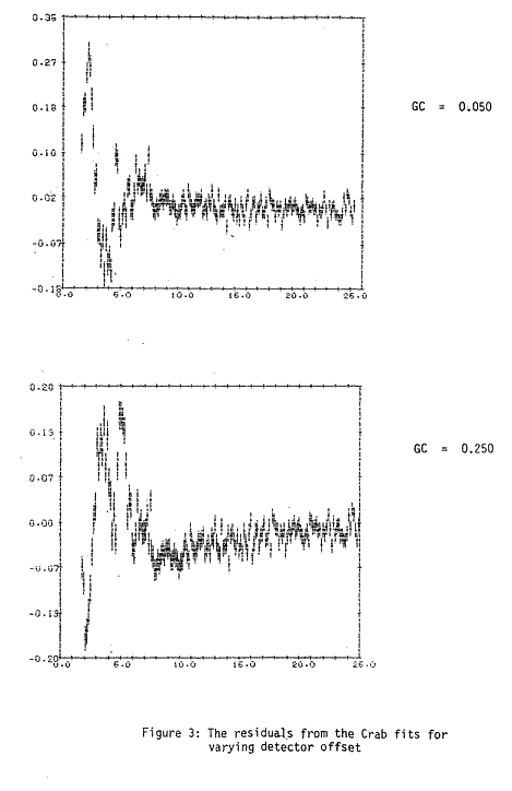
Appendix I contains a listing of a function PTAIL
which returns the probability of measuring in a given energy interval DE centered
on E a residual low energy tail from a photon with an initial energy
E1. It should be noted that the above function becomes undetermined at
E=E1. This is taken care of in PTAIL by integrating over the last
milli-percent of the function up to E1. The resulting line profile
should then be spread by the detector broadening function. In Figure 3 the
expected profile of a line injected at a single energy is illustrated. The second
peak is the escape peak. In the Observatory software to save computing time, the
low energy tail is not included on the escape peak. This will not make any
difference since the L-escape only represents < 3% of the total
count rate above 4.78 keV.
4. The Beryllium Window Thickness
The
pre-launch calculations assumed that the window had a constant thickness of 175
microns (the specified minimum). They, failed to take into account the fact that
the window is dome shaped and that the projected thickness increases towards the
edge of the dome (where most of the effective area is). Measurements on flight
spare windows indicated that thicknesses varied between 175 and 220 microns, and
the window thickness of the flight GSPC must at present be considered a free
parameter (within reasonable limits).
5. Edge Effects
Towards the edge of the
detector the electric field geometry becomes uncertain such that electron tracks
may be deflected to the detector walls and not registered. This area of the
detector is critical because it constitutes a large fraction of the total
effective area. In addition at this point the conical shaped detector walls meet
the dome shaped window ie. the total gas depth decreases to zero. This can cause
a fairly large L edge to appear in the response because photons just below the
edge have a higher probability of not being stopped than those just above it
where the penetration depth is low.
The fitting procedure described below indicated a
stronger L edge in the spectrum than would be expected. It could be removed to a
large extent by adjusting the detector parameters to take into account the
expected field geometry.
6. The Burst Length Efficiencies
Discrimination of events based on the rise time of the pulse generated (the burst
length) can be used to increase the signal to noise ratio, by reducing the
particle background counting rate. The optimum setting of the single channel
analyser discriminator is a trade-off, between the reduction in background and
the number of X-rays rejected and was established during the performance
verification phase as channels 89-107.
This results in a loss of between 10 and up to 90% of
the X-rays registered in the detector, with the fraction lost increasing rapidly
below 5 keV. The burst length discrimination efficiency as a function of energy
was determined during the February 1985 observation of the Crab by dividing the
burst length discrimination 89-107 spectrum by the 'no-discrimination' spectrum.
The data were smoothed and fit to a splined polynomial. The function GSAXE given
in Appendix II returns for a given energy E, the fraction of X-rays that are not
attenuated. The efficiencies are not well determined above ~15 keV because of
limitations in the background subtraction. However there appears to be no major
change in efficiency at higher energies and it is taken to be a constant. Also
given are the efficiencies for the 89-104 setting used early in the PV phase.
These efficiencies should be applied AFTER the
spreading by the detector response. Thus there will be only one set of effective
areas for all burst length window settings. (In the earlier calibration the burst
length efficiencies had been included in the initial effective areas because of
uncertainties in deconvolving these from the other problems in the detector
response).
7. Escape Fractions
A certain number of
photons emitted by the Xenon ions as they de-excite will escape the detector and
hence will cause a deficiency in the detected energy of precisely the energy of
the fluorescent photon. The efficiency of this process for the L shell of Xenon
is 3% at 5.1 keV, and decreases linearly to zero up to the K absorption edge. At
the K edge this then increases to 58% and is kept constant. The edge energies are
taken to be an average of the various sub-shells and are 5.1 keV (L) and 34.56
(K). Note the escape energy that must be subtracted is 4.33 keV and 30.49 keV
respectively.
8. Systematic Uncertainties
The main limiting factor
will always be the fact that the channel boundary widths are only known to 1%.
This means that a systematic error of 1% of the total count rate should be added
quadratically to the statistical error.
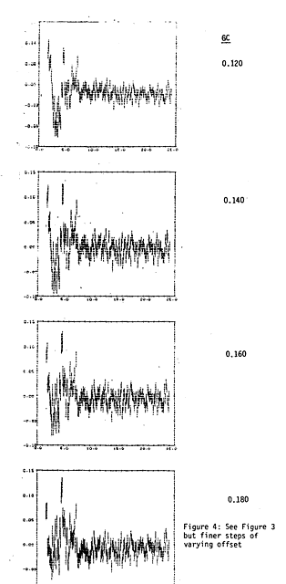
9. The Effective Areas and Zero Offset
The
above considerations leave two unknowns in the detector parameters: 1) The
average thickness of the window; 2) the energy offset of channel zero (when
referenced to energies above 4.78 keV). The effect of varying the zero offset on
fits to the Crab data without burst length discrimination was tested allowing the
window thickness to be a free parameter. The Crab spectrum was assumed to have an
energy index of 2.1 and a low energy cut-off of 3.5 x 10 21
H/cm2. Residuals from the fit using two different offsets of 50 eV and
250 eV are shown in Figure 3. The deviation from the fit in the lower channels
around 2-3 keV strongly depends on the chosen offset. When 50 eV is used there is
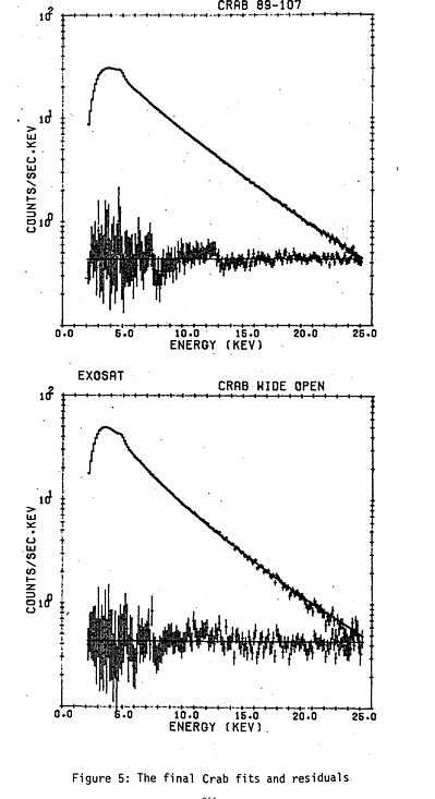
a strong excess of counts, whereas for 250 eV this becomes a deficit. In Figure 4
finer steps of varying offset are used. A reasonable fit to the data can be
obtained for an offset of 150 eV with an uncertainty of at most 50 eV in total.
This translates to plus or minus 25 eV at the iron line. The required window
thickness was ~200 microns.
There are still some small (< 2%), systematic trends
in the residuals left centered on 4.78 keV which can be attributed to edge
effects in the detector. Since these are very difficult to model they were
removed by fitting a polynomial to the response. The final residuals are shown in
Figure 5 along with the original PHA spectrum. Also given is the best fit to the
data obtained from the Crab using the 89-107 burst length setting. The final
overall effective areas fall short of the pre-launch values by ~15%. This is
ascribed to uncertainties in masking by the collimator support structures, edge
effects in the detector and count rate independent dead time effects (see 10). It
has been corrected by re-normalising the effective areas. In Appendix III the
current set of effective areas is listed.
These calibrations were then applied to the data on Cas A. The energy
of the Sulphur line is now consistent with that measured by the Einstein SSS. In
the case of the various different Crab observations, the new calibrations all
give in the 2-16 keV band (and where available the 2-30 keV band) a fit
consistent with a slope of 2.10 + 0.03 and a column density of 3.5 + 1.5 x
1021 H/cm 2 .
10. Dead Time
The accumulation times for
the Crab observations were corrected for data handling sampling effects using the
formula:
f = Co/(-S-Log(1.0 -
Co/S))
where Co is the observed count rate, and S is the
sampling rate in Hz given by the workspace parameter No.2 of all GSPC OBC
programs. The typical dead time is~0.7% for the background and ~5% for the Crab
(gain 2.0).
Additional 2.5% dead time effects (ref.
p.67) were not included for the Crab observations used to determine the GSPC
effective areas. Since these are count rate independent they were taken into
account during the re-normalisation of the effective areas to give the correct
normalisation for the Crab spectrum. Only the sampling effect should be included
when computing the dead time for spectral data. Note that the current CCF
backgrounds are not dead time corrected.
11. Outstanding Issues
A
self-consistent fit to the GSPC spectrum of the Crab can now be obtained up to a
level of a few percent. Any remaining uncertainties are most likely caused by
edge effects in the detector. The only improvement possible is in measuring the
burst length discrimination efficiency as a function of energy. The current
values become limited by uncertainties in the background subtraction, which may
lead to systematic variations at around the one percent level. This is well
within the quoted systematic uncertainties. A further set of observations of the
Crab will soon be carried out to better determine this parameter. However for all
purposes the current values are quite adequate and the difference will not be
noticed except for the very brightest sources (> 1 Crab).
There have been reports of problems with subtracting
the CCF background from recent data suggesting that the shape of the background
is varying. This may be because there is either a long term evolution with time
or a dependence with the absolute detector gain. A study of this problem is
currently underway and it is likely that a time/gain dependent CCF background
will be issued. In the meantime, users should compare the background obtained
from the slew file with that from the CCF. If there are obvious discrepancies, in
particular an excess or deficiency below channel 40 (gain 2.0), then two possible
solutions exist. First if the slew is long enough, use this as the background.
Otherwise, contact M. Gottwald for selection of a new background from an
observation close to the one in question.
12. New GSPC Operating Procedures
Two changes to the operation of the GSPC have been
made:
(1) The photomultiplier LED stimulations have
been discontinued except for one made before and after the high voltage has been
turned off. Experience has shown that the lead lines are quite adequate for
measuring the gain stability and that stimulations have a perverse habit of being
done when X-ray bursts or other interesting events occur.
(2) The standard gain mode is now gain 1.0. This is to accumulate
a time history of the background in gain 1.0 and to ensure that any (cyclotron)
line features in spectra above 15 keV are not missed. It should be noted that
this will in no way impact on measurements of the iron line which in gain 2.0 was
grossly oversampled (gain 1.0 gives 10 channels across a narrow iron line). The
only justification for using. gain 2.0 is for studying the Sulphur line in bright
supernova remnants, however no more observations of these objects (basically Cas
A and Tycho) are presently planned. If a user still feels strongly that gain 2.0
is best then a background observation carried out in gain 2.0 will be assigned on
the same orbit.
N.E. White
Appendix I
0001  FTN4,L
0002              FUNCTION PTAIL(ELINE,EOBS,DE)
0003  C
0004  C
0005  C          THIS FUNCTION PUTS IN THE LOW ENERGY
0006  C          TAIL IN THE GSPC RESPONSE        NEW JUNE 85
0007  C          SEE INOUE ET AL (1978) NUCL. INST. METHODS, 157, 295.
0008  C
0009  C
0010        DATA IJ/ 1 /
0011        IF (IJ.EQ.0) G0 TO 1
0012        AKMN = 0.03
0013        IJ = 0
0014    1   PTAIL = 0.0
0015  C
0016  C
0017        EEL = ELINE/5.9
0018        IF (ELINE.GT.10.) EEL = 1.69
0019        AK = AKMN / (EEL)**2.66667
0020        IF(ELINE.LT.4.78) AK = AK*0.348
0021        IF(ELINE.LT.5.10) AK = AK*0.710
0022        IF(ELINE.LT.5.45) AK = AK*0.860
0023  C
0024  C
0025  C
0026  C
0027    9  IF (EOBS.GE.O.9999*ELINE) G0 TO 8
0028       PTAIL = AK*(I-EOBS/ELINE)**(AK-I)*DE/ELINE
0029       RETURN
0030    8  PTAIL=(I.0-(EOBS-DE/2.0)/ELINE)-*AK
0031       RETURN
0032       END
Appendix II
0001 FTN4,L
0002       FUNCTION GSAXE(EIN,IBL)
0003 C
0004 C
0005 C THIS FUNCTION RETURNS THE BURST LENGTH EFFICIENCY AS A FUNCTION
0006 C OF ENERGY
0007 C
0008 C ACCEPTANCES IBL=0 WIDE OPEN
0009 C                 1 89-107
0010 C                 2 89-104
0011 C
0012 C
0013       DIMENSION E(S).POLI ( 13).POL2(13)
0014	   DATA E/0.0,15.0,28.0.88.0.188.0/
0015 C
0016 C
0017 C
0018 C 89-107/WO: SPLINE FIT TO-8S +84 CRAB DATA
0019 C
0020       DATA POL1/0.3.90.0.24SE-01, -0.1O5E-02,0.227E-04,0.I6OE-0I,
0021      *-0.122E-02 0.386E-04,0.578E-02,-0.630E-04,0.23SE-06,
0022      *0.129E-02,0.838E-04,-0.385E-05/
0023 C
0024 C
0025 C 89-1-04/WO
0026 C
0027       DATA POL2/0.322.0.184E-01,-0.969E-03.0.278E-04,0.153E-01
0028      *-0.133E-02,0.437E-04,0.543E-02,-0.36E-04.-O.197E-07,
0029      *0.270E-02,0.222E-04 -0.429E-O5/
0030 C
0031 C
0032 C
0033       DATA NMIN/12/,NMAX/100/
0034 C
0035 C
0036 C
0037       IF(IBL.NE.0)60 TO I
0038       GSAXE=1.0
0039       RETURN
0040       CONTINUE
0041       CHAN=(EIN-0.I5O)/0. 138792+0.5
0042       IF(CHAN.LT.NMIN)CHAN=NMIN
0043       IF(CHAN.GT.NMAX)CHAN=NMAX
0044       CHAN=CHAN-NMIN+I
0045       IF(IBL.EQ.I)CALL SPLIN(POLI,E,4,CHAN,GSAXE)
0046       IF(IBL.EQ.2)CALL SPLIN(POL2 E,4,CHAN,GSAXE)
0047       IF(GSAXE.GT.I.0-)GSAXE=I.0
0048       RETURN
0049       END

0001 FTN4,L
0002       SUBROUTINE SPLIN(P, E, N, EIN, VAL)
0003	   DIMENSION P(l),E(l)
0004	   VALP=P(l)
0005	   VAL=VALP
0006	   IF(EIN.LE.E(l))RETURN
0007	   DO 88 IV=I,N0
0008	   IF(EIR.GE.E(IV).AND.EIN.LT.E(IV+1))G0 TO 90
0009	   EE=E(IV+I)-E(IV)
0010	   VAL=VALP+POLY(P,EE,IV)
0011 88	   VALP=VAL
0012       IF(EIN.GT.E(N+I))RETURN
0013 90	   EE=EIN-E(IV)
0014       VAL=VALP+POLY(P,EE,IV)
0015	   RETURN
0016	   END
0017	   FUNCTION POLY(P,EE,IV)
0018	   DIMENSION P(1)
0019	   IN=(IV-I)*3+1
0020	   POLY=P(IN+l)*EE+P(IN+2)*EE*EE+P(IN+3)*EE*EE*EE
0021	   RETURN
0022	   END
Appendix III - GSPC Effective Areas
1 1.0000 .0000

2 1.1000 .0000

3 1.2000 .0001

4 1.3000 .0022

5 1.4000 .0170

6 1.5000 .0815

7 1.6000 .2757

8 1.7000 .7209

9 1.8000 1.6306

10 1.9000 3.1601

11 2.0000 5.4313

12 2.1000 8.4935

13 2.2000 12.3211

14 2.3000 16.8275

15 2.4000 21.8858

16 2.5000 27.3496

17 2.6000 33.0705

16 2.7000 38.9102

19 2.8000 44.7474

20 2.9000 56.4815

21 3.0000 56.0329

22 3.1000 61.3419

23 3.2000 66.3661

24 3.3000 71.0789

25 3.4000 75.4660

26 3.5OOO 79.5236

27 3.6000 83.2557

28 3.7000 66.6728

29 3.8000 89.7899

30 3.9000 92.6256

31 4.0000 95.2011

32 4.1000 97.5389

33 4.2000 99.6629

34 4.3000 101.5972

35 4.4000 103.3663

36 4.5000 104.9942

37 4.6000 107.5619

38 4.7000 111.6849

39 4.8000 121.0973

40 4.9000 122.6857

41 5.0000 119.4384

42 5.1000 121.7029

43 5.2000 122.8926

44 5.3000 123.9889

45 5.4000 124.9976

46 5.5000 126.3690

47 5.6000 127.2448

48 5.7000 128.0493

49 5.8000 128.7864

50 6.3000 131.5941

51 6.8000 133.2057

52 7.3000 133.8900

53 7.8000 133.8328

54 8.3000 133.1673

55 8.8000 131.9922

56 9.3000 130.3839

57 9.8000 128.4043

58 10.3000 126.4752

59 10.8000 124.5567

60 11.3000 122.4343

61 11.8000 120.1254

62 12.3000 117.6462

63 12.8000 115.0128

64 13.3000 112.2418

65 13.8000 109.3504

66 14.3000 106.3563

67 14.8000 103.2782

68 15.3000 100.1353

69 16.3000 93.7318

70 17.3000 87.2949

71 18.3000 80.9571

72 19.3000 74.8260

73 20.3000 68.9814

74 25.3000 45.1878

75 30.3000 29.8375

76 35.3000 78.1392

77 40.3000 64.3952

78 45.3000 52.6245

79 50.3000 42.9379

80 55.3000 35.1340

81 60.3000 28.9043

82 65.3000 23.9414

83 70.3000 19.9784

84 75.3000 16.7982
[EXOSAT Home]
[About EXOSAT]
[Archive]
[Software]
[Gallery]
[Publications]