Appendix B: Statistics in XSPEC

Introduction

There are two operations performed in XSPEC that require statistics. The first is parameter estimation, which comprises finding the parameters for a given model that provide the best fit to the data and then estimating uncertainties on these parameters. The second operation is testing whether the model and its best-fit parameters actually match the data. This is usually referred to as determining the goodness-of-fit.

Users can specify their statistic of choice with the statistic command. Which statistics should be used for these two operations depends on the probability distributions underlying the data. Almost all astronomical data are drawn from one of two distributions: Gaussian (or normal) and Poisson. The Poisson distribution is the familiar case of counting statistics and is valid whenever the only source of experimental noise is due to the number of events arriving at the detector. This is a good approximation for modern CCD instruments. If some other sort of noise is dominant then it is usually described by the Gaussian distribution. A common example of this is detectors that require background to be modeled in some way, rather than directly measured. The uncertainty in the background modeling is assumed to be Gaussian.

In the limit of large numbers of counts the Poisson distribution can be well approximated by a Gaussian so the latter is often used for detectors with high counting rates. In most cases this will cause no errors and does simplify the handling of background uncertainties however care should be exercised that no systematic offsets are introduced.

A fuller discussion of many of the issues discussed in this appendix can be found in Siemiginowska (2011).

Parameter Estimation

The standard statistic used in parameter estimation is the maximum likelihood. This is based on the intuitive idea that the best values of the parameters are those that maximize the probability of the observed data given the model. The likelihood is defined as the total probability of observing the data given the model and current parameters. In practice, the statistic used is twice the negative log likelihood.

Gaussian data (chi)

The likelihood for Gaussian data is

  $$L = \prod_{i=1}^N {1\over{\sigma_i\sqrt{2\pi}}} \exp\left[{{-(y_i-m_i)^2\over{2\sigma_i^2}}}\right]$$ (B.1)

where $y_i$ are the observed data rates, $\sigma_i$ their errors, and $m_i$ the values of the predicted data rates based on the model (with current parameters) and instrumental response. Taking twice the negative natural log of L and ignoring terms which depend only on the data (and will thus not change as parameters are varied) gives the familiar statistic :

  $$S^2 = \sum_{i=1}^N {(y_i-m_i)^2\over{\sigma_i^2}}$$ (B.2)

commonly referred to as chi-squared $\chi^2$ and used for the statistic chi option.

Gaussian data with background (chi)

The previous section assumed that the only contribution to the observed data was from the model. In practice, there is usually background. This can either be included in the model or taken from another spectrum file (read in using the backgrnd command). In the latter case the $y_i$ become observed data rates from the source spectrum subtracted by the background spectrum and the $\sigma_i$ are the source and background errors added in quadrature. Since the difference of two Gaussians variables is another Gaussian variable, the $S^2$ statistic can still be used in this case.

Poisson data (cstat)

The likelihood for Poisson distributed data is:

  $$L = \prod_{i=1}^N (tm_i)^{S_i} {\rm e}^{-tm_i}/S_i!$$ (B.3)

where $S_i$ are the observed counts, $t$ the exposure time, and $m_i$ the predicted count rates based on the current model and instrumental response. The maximum likelihood-based statistic for Poisson data, given in Cash (1979), is :

  $$C = 2\sum_{i=1}^N (tm_i) - S_i \ln{(tm_i)} + \ln{(S_i!)}$$ (B.4)

The final term depends only on the data (and hence makes no difference to the best-fit parameters) so can be replaced by Stirling's approximation to give :

  $$C = 2\sum_{i=1}^N (tm_i) - S_i + S_i (\ln{(S_i)} - \ln{(tm_i)})$$ (B.5)

which provides a statistic which asymptotes to $S^2$ in the limit of large number of counts (Castor, priv. comm.). This is what is used for the statistic cstat option. Note that using the $S^2$ statistic instead of $C$ is not recommended since it can produce biassed results even when the number of counts is quite large (see e.g. Humphrey et al. 2009).

If the statistic is specified as cstatN where N is an integer then the same formula is used except that the data and model are binned so that there are at least N counts in each bin. In general, this is not recommended since it is inefficient but can be useful when testing using simulations.

Poisson data with Poisson background (cstat)

This case is more difficult than that of Gaussian data because the difference between two Poisson variables is not another Poisson variable so the background data cannot be subtracted from the source and used within the C statistic. The combined likelihood for the source and background observations can be written as:

  $$L = \prod_{i=1}^N {(t_s(m_i+b_i))^{S_i}{\rm e}^{-t_s(m_i+b_i)}\over{S_i!}}\times{(t_bb_i)^{B_i}{\rm e}^{-t_bb_i}\over{B_i!}}$$ (B.6)

where $t_s$ and $t_b$ are the exposure times for the source and background spectra, respectively, $B_i$ are the background data and $b_i$ the predicted rates from a model for the expected background. Note that $b_i$ is the predicted background rate for the observation of the source. If the background is uniform and the source and background observations are extracted from different sized regions then $t_b$ should be the background observation exposure multiplied by the the ratio of the background to source region sizes. If there is a physically motivated model for the background then this likelihood can be used to derive a statistic which can be minimized while varying the parameters for both the source and background models.

As a simple illustration suppose the source spectrum is source.pha and the background spectrum back.pha. The source model is an absorbed apec and the background model is a power-law. Further suppose that the background model requires a different response matrix to the source, backmod.rsp say. The fit is set up by:

XSPEC12> data 1:1 source.pha 2:2 background.pha
XSPEC12> resp 2:1 backmod.rsp 2:2 backmod.rsp
XSPEC12> model phabs(apec)
XSPEC12> model 2:backmodel pow

where the normalization of the apec model is fixed to zero for the second data group (i.e. the background spectrum) and the parameters of the background model are linked between the data groups.

If there is no appropriate model for the background it is still possible to proceed. Suppose that each bin in the background spectrum is given its own parameter so that the background model is $b_i = f_i$ . A standard XSPEC fit for all these parameters would be impractical however there is an analytical solution for the best-fit $f_i$ in terms of the other variables which can be derived by using the fact that the derivative of $L$ will be zero at the best fit. Solving for the $f_i$ and substituting gives the profile likelihood:

  $$W/2 = \sum_{i=1}^N t_sm_i+(t_s+t_b)f_i-S_i\ln{(t_sm_i+t_sf_i)} -B_i\ln{(t_bf_i)}-S_i(1-\ln{S_i})-B_i(1-\ln{B_i})$$ (B.7)

where, if $(t_s+t_b)m_i-S_i-B_i) >= 0$ then

  $$f_i = {{2B_im_i}\over{(t_s+t_b)m_i-S_i-B_i+d_i}}$$ (B.8)

otherwise

  $$f_i = {{S_i+B_i-(t_s+t_b)m_i + d_i}\over{2(t_s+t_b)}}$$ (B.9)

and

  $$d_i = \sqrt{[(t_s+t_b)m_i-S_i-B_i]^2+4(t_s+t_b)B_im_i}$$ (B.10)

If any bin has $S_i$ and/or $B_i$ zero then its contribution to $W$ ($W_i$) is calculated as a special case. So, if $S_i$ is zero then:

  $$W_i/2 = t_sm_i-B_i\ln{(t_b/(t_s+t_b))}$$ (B.11)

If $B_i$ is zero then there are two special cases. If $m_i < S_i/(t_s+t_b)$ then:

  $$W_i/2 = -t_bm_i-S_i\ln{(t_s/(t_s+t_b))}$$ (B.12)

otherwise:

  $$W_i/2 = t_sm_i+S_i(\ln{S_i}-\ln{(t_sm_i)}-1)$$ (B.13)

This W statistic is used for statistic cstat if a background spectrum with Poisson statistics has been read in (note that in the screen output it will still be labeled as C statistic). In practice, it works well for many cases but for weak sources and small numbers of counts in the background spectrum it can generate an obviously wrong best fit. A possible solution is to bin the data to ensure every bin in the background spectrum contains enough counts (see https://giacomov.github.io/Bias-in-profile-poisson-likelihood/).

In the limit of large numbers of counts per spectrum bin a second-order Taylor expansion shows that $W$ tends to :

  $$\sum_{i=1}^N\left({[S_i-t_sm_i-t_sf_i]^2\over{t_s(m_i+f_i)}}+{[B_i-t_bf_i]^2\over{t_bf_i}}\right)$$ (B.14)

which is distributed as $\chi^2$ with ${\rm N} - {\rm M}$ degrees of freedom, where the model $m_i$ has M parameters (include the normalization).

Poisson data with Gaussian background (pgstat)

Another possible background option is if the background spectrum is not Poisson. For instance, it may have been generated by some model based on correlations between the background counts and spacecraft orbital position. In this case there may be an uncertainty associated with the background which is assumed to be Gaussian. In this case the same technique as above can be used to derive a profile likelihood statistic :

  $$PG = 2\sum_{i=1}^N t_s(m_i+f_i)-S_i\ln{(t_sm_i+t_sf_i)}+{1\over{2\sigma_i^2}}(B_i-t_bf_i)^2-S_i(1-\ln{S_i})$$ (B.15)

where

  $$f_i = {{-(t_s\sigma_i^2-t_bB_i+t_b^2m_i)\pm d_i}\over{2t_b^2}}$$ (B.16)

unless this gives $f_i < 0$ in which case

  $$f_i = 2{{t_s\sigma_i^2m_i-S_i\sigma_i^2-t_bB_im_i}\over{-(t_s\sigma_i^2-t_bB_i+t_b^2m_i)\pm d_i}}$$ (B.17)

and

  $$d_i = \sqrt{[t_s\sigma_i^2-t_bB_i+t_b^2m_i]^2-4t_b^2[t_s\sigma_i^2m_i-S_i\sigma_i^2-t_bB_im_i]}$$ (B.18)

The positive or negative square root is chosen depending on whether $t_s\sigma_i^2-t_bB_i+t_b^2m_i$ is greater than or less than zero, respectively.

There is a special case for any bin with $S_i$ equal to zero:

  $$PG_i = t_sm_i+B_i(t_s/t_b)-\sigma_i^2(t_s/t_b)^2/2$$ (B.19)

This is what is used for the statistic pgstat option.

Poisson data with known background (pstat)

Another possible background option is if the background spectrum is known. Again the same technique as above can be used to derive a profile likelihood statistic :

  $$P = 2\sum_{i=1}^N t_s(m_i+B_i/t_b)-S_i\ln{[t_s(m_i+B_i/t_b]}-S_i(1-\ln{S_i})$$ (B.20)

This is what is used for the statistic pstat option.

Bayesian analysis of Poisson data with Poisson background (lstat)

An alternative approach to fitting Poisson data with background is to use Bayesian methods. In this case instead of solving for the background rate parameters we marginalize over them writing the joint probability distribution of the source parameters as :

  $$P = p\left(\{\theta_j\}\vert\{S_i\},\{B_i\},I\right) = \int...\int \{db_k\}p\left(\{\theta_j\},\{b_k\}\vert\{S_i\},\{B_i\},I\right)$$ (B.21)

where $\{\theta_j\}$ are the source parameters, $\{b_k\}$ the background rate parameters and $I$ any prior information. Using Bayes theorem, that the $\{\theta_j\}$ and independent of the $\{b_k\}$, that the $\{b_k\}$ are individually independent and that the observed counts are Poisson gives :

  $$P = {p\left(\{\theta_j\}\vert I\right)\over{p\left(\{S_i\}\vert I... ...\right)}}\prod_{k=1}^N {t_s^{S_k}t_b^{B_k}{\rm e}^{-m_kt_s}\over{S_k!B_k!}}J_k$$ (B.22)

where :

  $$J_k = \int db_k p(b_k\vert I)(m_k+b_k)^{S_k}b_k^{B_k}{\rm e}^{-b_k(t_s+t_b)}$$ (B.23)

To calculate $J_k$ we need to make an assumption about the prior background probability distribution, $p(b_k\vert I)$. We follow Loredo (1992) and assume a uniform prior between 0 and $b_i^{max}$. Expanding the binomial gives :

  $$J_k = {1\over{b_k^{max}}}\sum_{j=0}^{S_k}m_k^j{S_k!\over{j!(S_k-j... ...mma\left(S_k+B_k-j+1,b_k^{max}(t_s+t_b)\right)}\over{(t_s+t_b)^{S_k+B_k-j+1}}}$$ (B.24)

where :

  $$\gamma(\alpha,\beta) = \int_0^{\beta} x^{(\alpha-1)}{\rm e}^{-x}dx$$ (B.25)

Again, following Loredo we assume that $(t_s+t_b)b_k^{max} >> B_k$ and using the approximation $\gamma(\alpha,\beta) \sim (\alpha-1)!$ when $\alpha >> \beta$ gives :

  $$J_k = {S_k!(t_s+t_b)^{-(S_k+B_k+1)}\over{b_k^{max}}}\sum_{j=0}^{S_k}m_k^j{(S_k+B_k-j)!\over{j!(S_k-j)!}}(t_s+t_b)^j$$ (B.26)

Note that for $m_k = 0$ only the $j = 0$ term in the summation is non-zero. Now, we define lstat by calculating $-2\ln{P}$ and ignoring all additive terms which are independent of the model parameters :

  $${\rm lstat} = -2\ln{p\left(\{\theta_j\}\vert I\right)}+2\sum_{k=1... ..._s-\ln{\sum_{j=0}^{S_k}m_k^j{(S_k+B_k-j)!\over{j!(S_k-j)!}}(t_s+t_b)^k}\right)$$ (B.27)

Including Bayesian priors

If Bayesian priors have been set using the bayes command then $-2\ln{P_{prior}}$ is added to the fit statistic value. The bayes documentation gives $\ln{P_{prior}}$ for each option.

Power spectra from time series data (whittle)

XSPEC has been used by a number of researchers to fit models to power spectra from time series data. In this case the x-axis is frequency (in Hz) and not keV so plots have to be modified appropriately. The correct fit statistic is that due to Whittle as discussed in Vaughan (2010) and Barret & Vaughan (2012) :

  $$S = 2\sum_{i=1}^N\left({y_i\over{m_i}}+\ln{m_i}\right)$$ (B.28)

Parameter confidence regions

Fisher Matrix

XSPEC provides several different methods to estimate the precision with which parameters are determined. The simplest, and least reliable, is based on the inverse of the second derivative of the statistic with respect to the parameter at the best fit. The first derivative must be zero by construction and the second derivative provides a measure of how rapidly the statistic increases away from the best-fit. The faster the statistic increases, i.e. the larger the second derivative, the more precisely the parameter is determined. The matrix of second derivatives is often referred to as the Fisher information. Its inverse is the covariance matrix, written out at the end of an XSPEC fit.

The +/- numbers provided for each parameter in the standard fit output are estimates of the one-sigma uncertainty, calculated as the square root of the diagonal elements of the covariance matrix. As such, these ignore any correlations between parameters. Whether correlations are important can be seen by comparing with the off-diagonal elements of the covariance matrix. In general, these estimates should be considered lower limits to the true uncertainty.

Correlation information is also given in the table of variances and principal axes which also appears at the end of a fit. Each row in this table is an eigenvalue and associated eigenvector of the Fisher matrix. If the parameters are independent then each eigenvector will have a contribution from only one parameter. For instance, if there are three independent parameters then the eigenvectors will be (1,0,0), (0,1,0), and (0,0,1). If the parameters are not independent then each eigenvector will show contributions from more than one parameter.

Delta Statistic

The next most reliable method for deriving parameter confidence regions is to find surfaces of constant delta statistic from the best-fit value, i.e. where :

  $${\rm Statistic} = {\rm Statistic_{best-fit}} + \Delta$$ (B.29)

This is the method used by the error command, which searches for the parameter value where the statistic differs from that at the best fit by a value ($\Delta$) specified in the command. For each value of the parameter being tested all other free parameters are allowed to vary. The results of the error command can be checked using steppar, which can also be used to find simultaneous confidence regions of multiple parameters. The specific values of $\Delta$ which generate particular confidence regions are calculated by assuming that it is distributed as chi-squared with the number of degrees of freedom equal to the number of parameters being tested (e.g. when using the error command there is one degree of freedom, when using steppar for two parameters followed by plot contour there are two degrees of freedom). This assumption is correct for the $S^2$ statistic and is asymptotically correct for other statistic choices.

Monte Carlo

The best but most computationally expensive methods for estimating parameter confidence regions are using two different Monte Carlo techniques. The first technique is to start with the best fit model and parameters and simulate datasets with identical properties (responses, exposure times, etc.) to those observed. For each simulation, perform a fit and record the best-fit parameters. The sets of best-fit parameters now map out the multi-dimensional probability distribution for the parameters assuming that the original best-fit parameters are the true ones. While this is unlikely to be true, the relative distribution should still be accurate so can be used to estimate confidence regions. There is no explicit command in XSPEC to use this technique however it is easy to construct scripts to perform the simulations and store the results.

The second technique is Markov Chain Monte Carlo (MCMC) and is of much wider applicability. In MCMC a chain of sets of parameter values is generated which describe the parameter probability distribution. This determines both the best-fit (the mode) and the confidence regions. The chain command runs MCMC chains which can be converted to probability distributions using margin (which takes the same arguments as steppar). The results can be plotted in 1- or 2-D using plot margin and plot integprob to plot the probability density and integrated probability. If MCMC chains are in use then the error command will use them to estimate the parameter uncertainty.

Goodness-of-fit

Parameter values and confidence regions only mean anything if the model actual fits the data. The standard way of assessing this is to perform a test to reject the null hypothesis that the observed data are drawn from the model. Thus we calculate some statistic $T$ and if $T_{obs} > T_{critical}$ then we reject the model at the confidence level corresponding to $T_{critical}$. Ideally, $T_{critical}$ is independent of the model so all that is required to evaluate the test is a table giving $T_{critical}$ values for different confidence levels. This is the case for chi-squared which is one of the reasons why it is used so widely. However, for other test statistics this may not be true and the distribution of $T$ must be estimated for the model in use then the observed value compared to that distribution. This is done in XSPEC using the goodness command. The model is simulated many times using parameter values drawn from the posterior probability distribution, each fake dataset is fit and a value of $T$ calculated. These are then ordered and a distribution constructed. This distribution can be plotted using plot goodness. Now suppose that $T_{obs}$ obs exceeds 90% of the simulated $T$ values we can reject the model at 90% confidence. For more discussion about the goodness command see the discussion on the Facebook xspec group.

It is worth emphasizing that goodness-of-fit testing only allows us to reject a model with a certain level of confidence, it never provides us with a probability that this is the correct model.

Chi-square (chi)

The standard goodness-of-fit test for Gaussian data is chisquared (as defined above).

Because the significance of the chi-squared values depends greatly upon the number of degrees of freedom (dof = number of data bins minus number of free parameters), Xspec does not print out the reduced chi-squared at the end of a fit. Instead, Xspec quotes the null hypothesis probability, which is the probability of the observed data being drawn from the model given the value of chi-squared and the dof. The dof is printed at the end of this line.

The chi-squared value is easily calculated, particularly while running from a script The tclout stat command returns the total fit statistic and tclout dof returns the number of degrees of freedom (and the number of channels). All that is left is the division.

A rough rule of thumb is that the chi-squared should be approximately equal to the dof. If the chi-squared is much greater than the dof then the observed data are likely not drawn from the model. If the chi-squared is much less than the dof then the Gaussian sigma associated with the data are likely over-estimated.

Pearson chi-square (pchi)

Pearson's original (1900) chi-square test was not for Gaussian data but for the case of dividing counts up between cells. This corresponds to the case of Poisson data with no background.

  $$\chi_P^2 = \sum_{i=1}^N {(y_i-m_i)^2\over{m_i}}$$ (B.30)

Kolmogorov-Smirnov (ks)

There are a number of test statistics based on the empirical distribution function (EDF). The EDF is the cumulative spectrum :

  $$Y_i = \left(\sum_{j=1}^iy_J\right)/\left(\sum_{j=1}^Ny_j\right)$$ (B.31)

for the data and

  $$M_i = \left(\sum_{j=1}^im_J\right)/\left(\sum_{j=1}^Nm_j\right)$$ (B.32)

for the model.

The EDF can be plotted using plot icounts. The best known of these tests is Kolmogorov-Smirnov whose statistic is simply the largest difference between the observed and model EDFs :

  $$D = supremum \vert Y_i-M_i\vert$$ (B.33)

The XSPEC statistic test ks option returns $\log{D}$. The significance of the ks value can be determined using the goodness command. In general, the Kolmogorov-Smirnov test is not particularly powerful and the next two test statistics are preferred.

Cramer-von Mises (cvm)

The Cramer-von Mises statistic is the sum of the squared differences of the EDFs :

  $$w^2 = \sum_{i=1}^N (Y_i-M_i)^2$$ (B.34)

The XSPEC statistic test cvm option returns $\log{w^2}$ and its significance should be determined using the goodness command.

Anderson-Darling (ad)

Anderson-Darling is a modification of Cramer-von Mises which places more weight on the tails of distribution :

  $$w^2 = \sum_{i=1}^N {(Y_i-M_i)^2\over{M_i(1-M_i)}}$$ (B.35)

The XSPEC statistic test ad option returns $\log{w^2}$ and its significance should be determined using the goodness command.

CUSUM (cusum)

The CUSUM statistic (Page, E.S. (1954, Biometrika, 41, 100)) is the difference between the largest and smallest differences between the model and data EFS.

  $$max(Y_i-M_i) - min(Y_i-M_i)$$ (B.36)

Runs (runs)

The Runs (or Wald-Wolfowitz) test checks that residuals are randomly distributed above and below zero and do not cluster. Suppose $N_p$ is the number of channels with +ve residuals, $N_n$ the number of channels with negative residuals, and $R$ the number of runs then the Runs statistic is :

  $$Runs = (R-\mu)/\sqrt{[(\mu-1)(\mu-2)/(N-1)]}$$ (B.37)

where :

  $$N = N_p + N_n$$ (B.38)

and

  $$\mu = {2N_pN_n\over{N}} + 1$$ (B.39)

The hypothesis that the residuals are randomly distributed can be rejected if abs(Runs) exceeds a critical value. For large sample runs (where $N_p$ and $N_n$ both exceed 10) the critical value is drawn from the Normal distribution. For instance, for a test at the 5% significance level, the hypothesis can be rejected if abs(Runs) exceeds 1.96.

Low Count Spectra

Using XSPEC on spectra with small numbers of counts per bin requires some care. In the following discussion we consider ways to ensure that we get an unbiased estimate of the parameters. We do not consider the problem of deciding whether the model with these parameters is a good fit.

Chi-squared : diagnostics and explanations

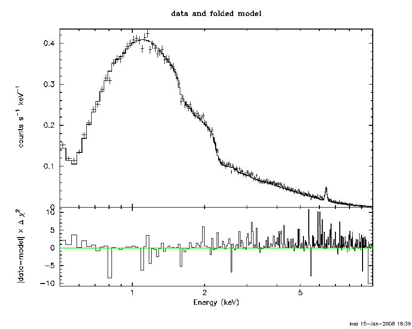
It is well-known that chi-squared doesn't work properly when there are significant numbers of bins in the spectrum with only a few counts. Folk wisdom is that there should be at least 5 counts in every bin. A good diagnostic for problems is if the best fit model is biased low relative to the data. The problems occur because the denominator in chi-squared is the variance for each bin. However, we don't necessarily know that variance so have to estimate it. The standard estimate is simply to use the data (assuming a Poisson distribution). Now, consider what happens if the data in a bin is an upward fluctuation or a downward fluctuation. Because we use the observed data as the denominator then a downward fluctuation contributes more to chi-squared than an upward fluctuation by the same amount. The net result is that the best-fit model is biased downwards.

For instance, this example in Fig B.1 shows that the data is systematically above the model at energies above 2 keV. Note that I binned up the plot using setplot rebin to make it look a bit better but this command does not bin the data used in the fit.

Figure B.1: Example using chi-squared.

Use cstat when there is no background

In the simple case where the background is non-existent or negligible and you can assume that the counts in a given channel are just a Poisson variable with mean given by the model-predicted counts in that channel then the best solution is to change the fit statistic to cstat (statistic cstat). The same model and response used above now gives the fit in Fig B.2 below which no longer has a downward bias at energies above 2 keV.

Figure B.2: Example using cstat.

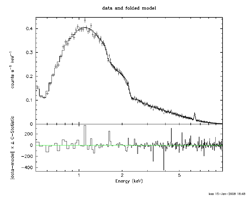
Confidence regions estimation proceeds in an identical fashion to that for the chi-squared statistic.

Here is an example of the effects of bias in chi-squared. Performing 1000 simulations of a Chandra spectrum with 1000 counts and a power-law index of 1.7 and then recovering the power-law index gives a mean and 90% range of

Standard chi-squared    1.41     (-0.15, +0.16) 
Gehrels chi-squared     1.88     (-0.22, +0.25) 
Churazov chi-squared    1.69     (-0.15, +0.16)  
Maximum Likelihood      1.70     (-0.13, +0.14)

When there is background it is more complicated

- Fit both the source and background files simultaneously

When possible, the best way to approach this is to simultaneously fit to both the source and background files with a background model for the background file and a combination of source model and background model for the source file. The parameters for the background models should be linked. A simple example would be set up in xspec as follows

XSPEC12>data 1:1 source.pi 2:2 background.pi
XSPEC12>model phabs(apec) + pow

where phabs(apec) is the source model and pow the background model. You will now be prompted for parameters for data group 1 (ie the source file) then data group 2 (ie the background file). For the second (background) set of parameters, freeze all the parameters of phabs(apec) and set the normalization to zero. Link the second set of parameters for the pow to the first set of parameters. Now fit using cstat.

The problems with this method are :

• It is somewhat cumbersome
• The background must have a known shape which can be modeled in xspec.

- Use a modified cstat

Xspec has a modified version of cstat (W, actually a profile likelihood, described above) for the case when there is a background file. Our simple example now becomes

XSPEC12>data source.pi 
XSPEC12>backgrnd background.pi
XSPEC12>model phabs(apec)

This works well in many cases however is known to fail sometimes when there are very few total counts in the spectrum. In this case, try grouping the spectrum so that there is at least one count in each bin. I have no idea why this helps but it does.

- Bin up the spectrum

An alternative approach is simply bin up the spectrum so that there are enough counts in each bin that the chi-squared bias is not significant. Note that this should be done using ftrbnpha or ftgrouppha, not within xspec using setplot rebin. Ideally, the binning scheme should not depend on the exact number of counts in each bin - ie the group constant option in ftgrouppha - but a deterministic scheme decided on before looking at the spectrum. This method has the obvious disadvantage that the binning erases information.

- Change the denominator in chi-squared

Since the problem with chi-squared arises because the estimator we use for the variance does not work well we can try a different estimator. One such scheme is to calculate an average number of counts over the surrounding spectral bins and use that as an estimator for the variance. This is done in xspec by changing the chi-squared weighting using the command weight churazov.

References

• Barret, D. & Vaughan, S., 2012. “Maximum likelihood fitting of X-ray power density spectra: application to high-frequency quasi-periodic oscillation from the neutron star X-ray binary 4U1608-522”, ApJ 746, 131.
• Cash, W., 1979. “Parameter estimation in astronomy through application of the likelihood ratio”, ApJ 228, 939.
• Humphrey, P.J., Liu, W. and Buote, D.A., “$\chi^2$ and Poissonian Data: Biases Even in the High-Count Regime and How to Avoid Them.”, ApJ 693, 822.
• Loredo, T., 1992. In “Statistical Challenges in Modern Astronomy”, eds. Feigelson, E.D. and Babu, G.J., pp 275-297.
• Siemiginowska, A., 2011. In “Handbook of X-ray Astronomy” eds. Arnaud, K.A., Smith, R.K. and Siemiginowska, A., Cambridge University Press, Cambridge.
• Vaughan, S. 2010, “A Bayesian test for periodic signals in red noise”, MNRAS 402, 307.

HEASARC Home | Observatories | Archive | Calibration | Software | Tools | Students/Teachers/Public

Last modified: Friday, 23-Aug-2024 13:20:40 EDT

HEASARC Staff Scientist Position - Applications are now being accepted for a Staff Scientist with significant experience and interest in the technical aspects of astrophysics research, to work in the High Energy Astrophysics Science Archive Research Center (HEASARC) at NASA Goddard Space Flight Center (GSFC) in Greenbelt, MD. Refer to the AAS Job register for full details.