
Come analyze HEASARC, IRSA, and MAST data in the cloud! The Fornax Initiative is now welcoming all interested beta users.


Parameter Estimation
The standard statistic used in parameter estimation is the maximum likelihood. This is based on the intuitive idea that the best values of the parameters are those that maximize the probability of the observed data given the model. The likelihood is defined as the total probability of observing the data given the model and current parameters. In practice, the statistic used is twice the negative log likelihood.
Gaussian data (chi)
The likelihood for Gaussian data is
![$\displaystyle L = \prod_{i=1}^N {1\over{\sigma_i\sqrt{2\pi}}}
\exp\left[{{-(y_i-m_i)^2\over{2\sigma_i^2}}}\right]$](img712.svg) |
(B.1) |
where  are the observed data rates,
  their errors, and
  the
values of the predicted data rates based on the model (with current
parameters) and instrumental response. Taking twice the negative
natural log of L and ignoring terms which depend only on the data (and
will thus not change as parameters are varied) gives the familiar
statistic :
the
values of the predicted data rates based on the model (with current
parameters) and instrumental response. Taking twice the negative
natural log of L and ignoring terms which depend only on the data (and
will thus not change as parameters are varied) gives the familiar
statistic :
 |
(B.2) |
commonly referred to as chi-squared  and used for the statistic chi option.
Gaussian data with background (chi)
The previous section assumed that the only contribution to the
observed data was from the model. In practice, there is usually
background. This can either be included in the model or taken from
another spectrum file (read in using the backgrnd command). In the latter
case the become observed data rates from the source spectrum
subtracted by the background spectrum and the are the source and
background errors added in quadrature. Since the difference of two
Gaussians variables is another Gaussian variable, the  statistic can
still be used in this case.
statistic can
still be used in this case.
Poisson data (cstat)
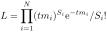
The likelihood for Poisson distributed data is:
 |
(B.3) |
where  are the observed counts,
  the exposure time, and
the predicted count rates based on the current model and instrumental
response. The maximum likelihood-based statistic for Poisson data,
given in Cash (1979), is :
the exposure time, and
the predicted count rates based on the current model and instrumental
response. The maximum likelihood-based statistic for Poisson data,
given in Cash (1979), is :
 |
(B.4) |
The final term depends only on the data (and hence makes no difference to the best-fit parameters) so can be replaced by Stirling's approximation to give :
 |
(B.5) |
which provides a statistic which asymptotes to in the limit of large
number of counts (Castor, priv. comm.). This is what is used for the
statistic cstat option. Note that using the statistic
instead of  is not recommended since it can produce biassed results
even when the number of counts is quite large (see
e.g. Humphrey et al. 2009).
is not recommended since it can produce biassed results
even when the number of counts is quite large (see
e.g. Humphrey et al. 2009).
Earlier versions accepted cstatN, where N is an integer, which applied the same formula after binning the data and model to at least N counts per bin. That option has been removed — the threshold it applied was N divided by the exposure time rather than N counts, and the binning was not carried through to the derivatives or the degrees of freedom. Group the data first instead (the group command, or an external tool such as ftgrouppha) and use plain cstat.
Poisson data with Poisson background (cstat)
This case is more difficult than that of Gaussian data because the difference between two Poisson variables is not another Poisson variable so the background data cannot be subtracted from the source and used within the C statistic. The combined likelihood for the source and background observations can be written as:
 |
(B.6) |
where  and
and  are the exposure times for the source and
background spectra, respectively,
are the exposure times for the source and
background spectra, respectively,  are the background data and
  the predicted rates from a model for the expected background. Note
that is the predicted background rate for the observation of the
source. If the background is uniform and the source and background
observations are extracted from different sized regions then
should be the background observation exposure multiplied by the the
ratio of the background to source region sizes. If there
is a physically motivated model for the background then this
likelihood can be used to derive a statistic which can be minimized
while varying the parameters for both the source and background
models.
the predicted rates from a model for the expected background. Note
that is the predicted background rate for the observation of the
source. If the background is uniform and the source and background
observations are extracted from different sized regions then
should be the background observation exposure multiplied by the the
ratio of the background to source region sizes. If there
is a physically motivated model for the background then this
likelihood can be used to derive a statistic which can be minimized
while varying the parameters for both the source and background
models.
As a simple illustration suppose the source spectrum is source.pha and the background spectrum back.pha. The source model is an absorbed apec and the background model is a power-law. Further suppose that the background model requires a different response matrix to the source, backmod.rsp say. The fit is set up by:
XSPEC> data 1:1 source.pha 2:2 background.pha
XSPEC> resp 2:1 backmod.rsp 2:2 backmod.rsp
XSPEC> model phabs(apec)
XSPEC> model 2:backmodel pow
where the normalization of the apec model is fixed to zero for the second data group (i.e. the background spectrum) and the parameters of the background model are linked between the data groups.
If there is no appropriate model for the background it is still
possible to proceed. Suppose that each bin in the background spectrum
is given its own parameter so that the background model is  . A
standard XSPEC fit for all these parameters would be impractical
however there is an analytical solution for the best-fit
. A
standard XSPEC fit for all these parameters would be impractical
however there is an analytical solution for the best-fit  in terms
of the other variables which can be derived by using the fact that the
derivative of
in terms
of the other variables which can be derived by using the fact that the
derivative of  will be zero at the best fit. Solving for the and
substituting gives the profile likelihood:
will be zero at the best fit. Solving for the and
substituting gives the profile likelihood:
 |
(B.7) |
where, if
 then
then
 |
(B.8) |
otherwise
 |
(B.9) |
and
![$\displaystyle d_i = \sqrt{[(t_s+t_b)m_i-S_i-B_i]^2+4(t_s+t_b)B_im_i}$](img733.svg) |
(B.10) |
If any bin has and/or zero then its contribution to  (
( ) is calculated
as a special case. So, if is zero then:
) is calculated
as a special case. So, if is zero then:
 |
(B.11) |
If is zero then there are two special cases. If
 then:
then:
 |
(B.12) |
otherwise:
 |
(B.13) |
This W statistic is used for statistic cstat if a background spectrum with Poisson statistics has been read in (note that in the screen output it will still be labeled as C statistic). In practice, it works well for many cases but for weak sources and small numbers of counts in the background spectrum it can generate an obviously wrong best fit. A possible solution is to bin the data to ensure every bin in the background spectrum contains enough counts (see https://zerohypeai.substack.com/bias-in-profile-poisson-likelihood/).
In the limit of large numbers of counts per spectrum bin a
second-order Taylor expansion shows that tends to :
![$\displaystyle \sum_{i=1}^N\left({[S_i-t_sm_i-t_sf_i]^2\over{t_s(m_i+f_i)}}+{[B_i-t_bf_i]^2\over{t_bf_i}}\right)$](img740.svg) |
(B.14) |
which is distributed as with
 degrees of freedom, where
the model has M parameters (including the normalization).
degrees of freedom, where
the model has M parameters (including the normalization).
Grouping the background on top of the source (cstat)
The wrong best fits noted above arise because the W statistic carries one free
background rate for every source bin: as the data grow so does the number
of these nuisance parameters, and for a sparse background their noise biases
the source parameters (a Neyman–Scott incidental-parameters problem). XSPEC
can suppress this by grouping the background on top of the current
source binning. The source bins are gathered into a smaller number of
“super-bins”, and a single background rate is shared by all the source bins
within a super-bin. The grouping is hierarchical — each super-bin is a
contiguous block of whole source bins and so cannot cut across the source
binning — and is set at run time with the group back command
(q.v.). A GROUPING column carried by the background spectrum file is not used
for this: on input XSPEC applies the source grouping to the background and
ignores any grouping of the background file.
Let the  source bins be partitioned into
  super-bins, with super-bin
  containing the
  source bins
  (so
(so
 ) and carrying a
single background rate
) and carrying a
single background rate  . Writing
 for the pooled
background counts of the super-bin, the profile likelihood generalises to
for the pooled
background counts of the super-bin, the profile likelihood generalises to
![$\displaystyle W/2 = \sum_{k=1}^{K}\left[\,\sum_{i\in k}\Big(t_sm_i+t_sf_k-S_i\ln{(t_sm_i+t_sf_k)}\Big)
+ n_kt_bf_k - B_k\ln{(t_bf_k)} + C_k\right]$](img747.svg) |
(B.15) |
where  collects the same data-only constant terms as before. The shared
rate is the root of the pooled score equation
collects the same data-only constant terms as before. The shared
rate is the root of the pooled score equation
 |
(B.16) |
which XSPEC solves by Newton-Raphson because, for  , the sum over source
bins with different has no closed form. When
, the sum over source
bins with different has no closed form. When  the equation reduces
to the per-bin quadratic for given above, so an ungrouped background
recovers the standard W statistic exactly; the
the equation reduces
to the per-bin quadratic for given above, so an ungrouped background
recovers the standard W statistic exactly; the  and
and  special
cases are handled as before. Pooling shrinks the number of profiled background
parameters from to , which is what reduces the bias for faint sources on
a sparse background. The same pooled treatment is applied to the other
statistics that profile or marginalize a per-bin background rate
(pgstat, lstat).
special
cases are handled as before. Pooling shrinks the number of profiled background
parameters from to , which is what reduces the bias for faint sources on
a sparse background. The same pooled treatment is applied to the other
statistics that profile or marginalize a per-bin background rate
(pgstat, lstat).
Poisson data with Gaussian background (pgstat)
Another possible background option is if the background spectrum is not Poisson. For instance, it may have been generated by some model based on correlations between the background counts and spacecraft orbital position. In this case there may be an uncertainty associated with the background which is assumed to be Gaussian. In this case the same technique as above can be used to derive a profile likelihood statistic :
 |
(B.17) |
where
 |
(B.18) |
unless this gives  in which case
 |
(B.19) |
and
![$\displaystyle d_i = \sqrt{[t_s\sigma_i^2-t_bB_i+t_b^2m_i]^2-4t_b^2[t_s\sigma_i^2m_i-S_i\sigma_i^2-t_bB_im_i]}$](img758.svg) |
(B.20) |
The positive or negative square root is chosen depending on whether
 is greater than or less than zero, respectively.
There is a special case for any bin with equal to zero:
 |
(B.21) |
This is what is used for the statistic pgstat option.
Poisson data with known background (pstat)
Another possible background option is if the background spectrum is known. Again the same technique as above can be used to derive a profile likelihood statistic :
![$\displaystyle P = 2\sum_{i=1}^N t_s(m_i+B_i/t_b)-S_i\ln{[t_s(m_i+B_i/t_b]}-S_i(1-\ln{S_i})$](img761.svg) |
(B.22) |
This is what is used for the statistic pstat option.
Bayesian analysis of Poisson data with Poisson background (lstat)
An alternative approach to fitting Poisson data with background is to use Bayesian methods. In this case instead of solving for the background rate parameters we marginalize over them writing the joint probability distribution of the source parameters as :
 |
(B.23) |
where
 are the source parameters,
  the
background rate parameters and
the
background rate parameters and  any prior information. Using Bayes
theorem, that the
and independent of the , that the are
individually independent and that the observed counts are Poisson gives :
any prior information. Using Bayes
theorem, that the
and independent of the , that the are
individually independent and that the observed counts are Poisson gives :
 |
(B.24) |
where :
 |
(B.25) |
To calculate  we need to make an assumption about the prior
background probability distribution,
we need to make an assumption about the prior
background probability distribution, 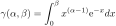 . We follow Loredo (1992)
and assume a uniform prior between 0 and
. We follow Loredo (1992)
and assume a uniform prior between 0 and  . Expanding the binomial
gives :
. Expanding the binomial
gives :
 |
(B.26) |
where :
 |
(B.27) |
Again, following Loredo we assume that
 and
using the approximation
and
using the approximation
 when
when
 gives :
 |
(B.28) |
Note that for  only the
  term in the summation is
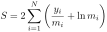
non-zero. Now, we define lstat by calculating
term in the summation is
non-zero. Now, we define lstat by calculating  and ignoring all
additive terms which are independent of the model parameters :
and ignoring all
additive terms which are independent of the model parameters :
 |
(B.29) |
Including Bayesian priors
If Bayesian priors have been set using the bayes command then
 is added to the fit statistic
value. The bayes documentation gives
is added to the fit statistic
value. The bayes documentation gives
 for each option.
Power spectra from time series data (whittle)
XSPEC has been used by a number of researchers to fit models to power spectra from time series data. In this case the x-axis is frequency (in Hz) and not keV so plots have to be modified appropriately. The correct fit statistic is that due to Whittle as discussed in Vaughan (2010) and Barret & Vaughan (2012) :
 |
(B.30) |
If the statistic is given as whittle with a number appended (e.g. whittle5) then the statistic is appropriate for that number of power density functions averaged together.
Correlated spectra (chistokes / chicov)
The statistics above all assume that the spectra being fit are independent: the variance of each bin enters on its own and there are no cross terms between spectra. This breaks down when several spectra are correlated bin-by-bin. The motivating case is spectropolarimetry: the Stokes I, Q and U spectra of a source with non-negligible polarization are extracted from the same events and are correlated, so fitting Q and U as if they were independent Gaussians is formally incorrect. The same situation arises whenever spectra share photons — overlapping or mosaicked extraction regions, neighbouring grating orders, or correlated detectors. The chistokes statistic (and its general alias chicov) handle these cases by carrying a per-bin covariance between spectra and using it in a multivariate-Gaussian likelihood.
The correlated spectra form a covariance group of  members. For each spectral bin
  there is an
  symmetric
covariance matrix
symmetric
covariance matrix  among the members. Its diagonal is the
ordinary per-bin variance of each member and its off-diagonal elements
are the cross-spectrum covariances; these are read from the data files
(see the format note below). Writing
among the members. Its diagonal is the
ordinary per-bin variance of each member and its off-diagonal elements
are the cross-spectrum covariances; these are read from the data files
(see the format note below). Writing  for the vector of residuals
 over the group members at bin , twice the negative log of the
multivariate-Gaussian likelihood gives, after dropping data-only
constants,
over the group members at bin , twice the negative log of the
multivariate-Gaussian likelihood gives, after dropping data-only
constants,
 |
(B.31) |
which reduces exactly to chi-squared when is diagonal. The
matrix is data-derived and does not depend on the model, so the
gradient is exact,
 |
(B.32) |
and is used by the fit. Each bin is solved by a Cholesky
factorization of (the cost is negligible because is
small).
A covariance estimated from a finite number of events need not be
positive definite. When the Cholesky factorization fails XSPEC keeps
the diagonal (the variances) exact and scales the whole off-diagonal
block by a factor  , where
  is chosen so that the
repaired bin is usably conditioned, i.e. the determinant of its
correlation matrix is at least
is chosen so that the
repaired bin is usably conditioned, i.e. the determinant of its
correlation matrix is at least  , bounding the amplification of the
quadratic form at about ten times the independent-Gaussian value, for
any number of members. As
, bounding the amplification of the
quadratic form at about ten times the independent-Gaussian value, for
any number of members. As
 the bin degrades gracefully to
the independent-Gaussian (ordinary chi-squared) contribution.
A bin whose variance is itself non-positive is dropped, as is a bin
whose supplied covariance is positive definite but numerically
degenerate (correlation determinant below
the bin degrades gracefully to
the independent-Gaussian (ordinary chi-squared) contribution.
A bin whose variance is itself non-positive is dropped, as is a bin
whose supplied covariance is positive definite but numerically
degenerate (correlation determinant below  ); the latter is
valid input that is merely unusable, and is reported rather than
silently weakened. The number of shrunk and
dropped bins is reported at the end of the fit; a group that needs
heavy shrinkage in many bins usually has a poorly estimated covariance
(too few counts) and should be binned more coarsely.
); the latter is
valid input that is merely unusable, and is reported rather than
silently weakened. The number of shrunk and
dropped bins is reported at the end of the fit; a group that needs
heavy shrinkage in many bins usually has a poorly estimated covariance
(too few counts) and should be binned more coarsely.
Active sub-block. The fit statistic is assigned per spectrum, so
a covariance group need not be fit entirely with chicov. The
statistic operates only on the sub-matrix of over the
members currently assigned chistokes/chicov; members
assigned another statistic (for example a low-count Stokes I fit with
cstat) are fit independently by that statistic and are simply
absent from the sub-block. The owner that evaluates the joint term is
the lowest-numbered active member; the others contribute nothing
themselves. Thus a Stokes set extracted as three members can be fit as
“cstat on I, chicov on Q and U” (the  Q–U sub-block, identical to the original Q–U treatment) or as
“chicov on I, Q and U” (the full
Q–U sub-block, identical to the original Q–U treatment) or as
“chicov on I, Q and U” (the full  ) with no
re-extraction — only the statistic assignment changes. For the Stokes
the I–Q and I–U covariances are second order in the
polarization fraction and negligible at typical (few per cent)
polarizations, so the two choices give the same fitted polarization;
the is therefore mainly a correctness check on the general
machinery, whose real value is genuinely correlated multi-spectrum
cases.
) with no
re-extraction — only the statistic assignment changes. For the Stokes
the I–Q and I–U covariances are second order in the
polarization fraction and negligible at typical (few per cent)
polarizations, so the two choices give the same fitted polarization;
the is therefore mainly a correctness check on the general
machinery, whose real value is genuinely correlated multi-spectrum
cases.
Because the covariance is bin-to-bin, all members of a group must share an identical grouping and be noticed identically, and the statistic range given to the statistic command must cover every active member of the group (XSPEC refuses the fit otherwise). For Stokes data the correct workflow is to choose the grouping on the high-count I spectrum (e.g. optimal Kaastra–Bleeker binning) and copy the identical GROUPING array to Q and U; the signed Q and U spectra must never be grouped on their own.
File format. Covariances are carried in the member spectrum files
as an OGIP-style local convention marked by the keyword
COVFRMT='XCOV-SET-1'. Each member also carries
COVGRP (a string group identifier shared by all members),
COVIDX (the 1-based member index) and NCOVMEM (the
number of members). The off-diagonal covariances are stored in an
upper-triangle layout: member holds one column
XCOV for each partner
  , giving the per-bin
covariance between members and . For a Stokes set with
, giving the per-bin
covariance between members and . For a Stokes set with
 ,
,
 ,
,
 the I file holds
XCOV2 (I–Q) and XCOV3 (I–U), the Q file holds
XCOV3 (Q–U), and the U file holds none. Older Q–U pair files
written by the original implementation (marked
COVFRMT='XCOV-PAIR-1' with a bare XCOV column and an
XCOVSIB sibling keyword) are auto-promoted to a two-member
group on load, so existing extractions continue to work unchanged. The
ftextractor tool writes Q–U pairs by default and the full I,Q,U
group with stokescov=iqu; the grouping is applied with
ftgrouppha, which sums the XCOV columns alongside the counts.
the I file holds
XCOV2 (I–Q) and XCOV3 (I–U), the Q file holds
XCOV3 (Q–U), and the U file holds none. Older Q–U pair files
written by the original implementation (marked
COVFRMT='XCOV-PAIR-1' with a bare XCOV column and an
XCOVSIB sibling keyword) are auto-promoted to a two-member
group on load, so existing extractions continue to work unchanged. The
ftextractor tool writes Q–U pairs by default and the full I,Q,U
group with stokescov=iqu; the grouping is applied with
ftgrouppha, which sums the XCOV columns alongside the counts.
Simulation. The fakeit, sim and goodness
commands draw correlated data for a covariance group rather than treating
its members independently. For each bin the member-residual vector is drawn
as  , where
  is a standard normal vector and
 is the Cholesky factorization of the same per-bin covariance (including any
off-diagonal shrinkage) that the statistic uses; the result is added to the
folded model. This is the forward dual of the
is the Cholesky factorization of the same per-bin covariance (including any
off-diagonal shrinkage) that the statistic uses; the result is added to the
folded model. This is the forward dual of the
 the
statistic evaluates, so simulated datasets follow the correct
distribution and goodness p-values are valid. This happens
automatically whenever the members carry covariance columns and are assigned
chistokes/chicov; a group member assigned an ordinary
per-spectrum statistic (e.g. I under cstat) is drawn independently.
All members must be Gaussian (a Poisson member raises an error). A
fakeit of a covariance group propagates the group keywords and the
XCOV columns to the output spectra; as with any fakeit the
output is ungrouped, so apply the grouping (which sums the XCOV
columns) before fitting the faked data with chicov.
the
statistic evaluates, so simulated datasets follow the correct
distribution and goodness p-values are valid. This happens
automatically whenever the members carry covariance columns and are assigned
chistokes/chicov; a group member assigned an ordinary
per-spectrum statistic (e.g. I under cstat) is drawn independently.
All members must be Gaussian (a Poisson member raises an error). A
fakeit of a covariance group propagates the group keywords and the
XCOV columns to the output spectra; as with any fakeit the
output is ungrouped, so apply the grouping (which sums the XCOV
columns) before fitting the faked data with chicov.
Fisher Matrix
XSPEC provides several different methods to estimate the precision with which parameters are determined. The simplest, and least reliable, is based on the inverse of the second derivative of the statistic with respect to the parameter at the best fit. The first derivative must be zero by construction and the second derivative provides a measure of how rapidly the statistic increases away from the best-fit. The faster the statistic increases, i.e. the larger the second derivative, the more precisely the parameter is determined. The matrix of second derivatives is often referred to as the Fisher information. Its inverse is the covariance matrix, written out at the end of an XSPEC fit.
The +/- numbers provided for each parameter in the standard fit output are estimates of the one-sigma uncertainty, calculated as the square root of the diagonal elements of the covariance matrix. As such, these ignore any correlations between parameters. Whether correlations are important can be seen by comparing with the off-diagonal elements of the covariance matrix. In general, these estimates should be considered lower limits to the true uncertainty.
Correlation information is also given in the table of variances and principal axes which also appears at the end of a fit. Each row in this table is an eigenvalue and associated eigenvector of the Fisher matrix. If the parameters are independent then each eigenvector will have a contribution from only one parameter. For instance, if there are three independent parameters then the eigenvectors will be (1,0,0), (0,1,0), and (0,0,1). If the parameters are not independent then each eigenvector will show contributions from more than one parameter.
Delta Statistic
The next most reliable method for deriving parameter confidence regions is to find surfaces of constant delta statistic from the best-fit value, i.e. where :
 |
(B.33) |
This is the method used by the error command, which searches for the
parameter value where the statistic differs from that at the best fit
by a value ( ) specified in the command. For each value of the
parameter being tested all other free parameters are allowed to
vary. The results of the error command can be checked using steppar,
which can also be used to find simultaneous confidence regions of
multiple parameters. The specific values of which generate
particular confidence regions are calculated by assuming that it is
distributed as chi-squared with the number of degrees of freedom equal to the
number of parameters being tested (e.g. when using the error command
there is one degree of freedom, when using steppar for two parameters
followed by plot contour there are two degrees of freedom). This
assumption is correct for the statistic and is asymptotically
correct for other statistic choices.
) specified in the command. For each value of the
parameter being tested all other free parameters are allowed to
vary. The results of the error command can be checked using steppar,
which can also be used to find simultaneous confidence regions of
multiple parameters. The specific values of which generate
particular confidence regions are calculated by assuming that it is
distributed as chi-squared with the number of degrees of freedom equal to the
number of parameters being tested (e.g. when using the error command
there is one degree of freedom, when using steppar for two parameters
followed by plot contour there are two degrees of freedom). This
assumption is correct for the statistic and is asymptotically
correct for other statistic choices.
Monte Carlo
The best but most computationally expensive methods for estimating parameter confidence regions are using two different Monte Carlo techniques. The first technique is to start with the best fit model and parameters and simulate datasets with identical properties (responses, exposure times, etc.) to those observed. For each simulation, perform a fit and record the best-fit parameters. The sets of best-fit parameters now map out the multi-dimensional probability distribution for the parameters assuming that the original best-fit parameters are the true ones. While this is unlikely to be true, the relative distribution should still be accurate so can be used to estimate confidence regions. There is no explicit command in XSPEC to use this technique however it is easy to construct scripts to perform the simulations and store the results.
The second technique is Markov Chain Monte Carlo (MCMC) and is of much wider applicability. In MCMC a chain of sets of parameter values is generated which describe the parameter probability distribution. This determines both the best-fit (the mode) and the confidence regions. The chain command runs MCMC chains which can be converted to probability distributions using margin (which takes the same arguments as steppar). The results can be plotted in 1- or 2-D using plot margin and plot integprob to plot the probability density and integrated probability. If MCMC chains are in use then the error command will use them to estimate the parameter uncertainty.