
Come analyze HEASARC, IRSA, and MAST data in the cloud! The Fornax Initiative is now welcoming all interested beta users.


Goodness-of-fit
Parameter values and confidence regions only mean anything if the
model actually fits the data. The standard way of assessing this is to
perform a test to reject the null hypothesis that the observed data
are drawn from the model. Thus we calculate some statistic  and if
 then we reject the model at the confidence
level corresponding to
then we reject the model at the confidence
level corresponding to
 . Ideally,
is
independent of the model so all that is required to evaluate the test
is a table giving
values for different confidence
levels. This is the case for chi-squared which is one of the reasons why
it is used so widely. However, for other test statistics this may not
be true and the distribution of must be estimated for the model in
use then the observed value compared to that distribution. This is
done in XSPEC using the goodness command. The model is simulated
many times using parameter values drawn from the posterior probability
distribution, each fake dataset is fit and a value of
calculated. These are then ordered and a distribution
constructed. This distribution can be plotted using plot goodness.
Now suppose that
. Ideally,
is
independent of the model so all that is required to evaluate the test
is a table giving
values for different confidence
levels. This is the case for chi-squared which is one of the reasons why
it is used so widely. However, for other test statistics this may not
be true and the distribution of must be estimated for the model in
use then the observed value compared to that distribution. This is
done in XSPEC using the goodness command. The model is simulated
many times using parameter values drawn from the posterior probability
distribution, each fake dataset is fit and a value of
calculated. These are then ordered and a distribution
constructed. This distribution can be plotted using plot goodness.
Now suppose that 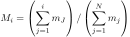 exceeds 90% of the
simulated values we can reject the model at 90% confidence. For
more discussion about the goodness command see the discussion
on the Facebook xspec group.
exceeds 90% of the
simulated values we can reject the model at 90% confidence. For
more discussion about the goodness command see the discussion
on the Facebook xspec group.
It is worth emphasizing that goodness-of-fit testing only allows us to reject a model with a certain level of confidence, it never provides us with a probability that this is the correct model.
Chi-square (chi)
The standard goodness-of-fit test for Gaussian data is chisquared (as defined above).
Because the significance of the chi-squared values depends greatly upon the number of degrees of freedom (dof = number of data bins minus number of free parameters), Xspec does not print out the reduced chi-squared at the end of a fit. Instead, Xspec quotes the null hypothesis probability, which is the probability of the observed data being drawn from the model given the value of chi-squared and the dof. The dof is printed at the end of this line.
The chi-squared value is easily calculated, particularly while running from a script The tclout stat command returns the total fit statistic and tclout dof returns the number of degrees of freedom (and the number of channels). All that is left is the division.
A rough rule of thumb is that the chi-squared should be approximately equal to the dof. If the chi-squared is much greater than the dof then the observed data are likely not drawn from the model. If the chi-squared is much less than the dof then the Gaussian sigma associated with the data are likely over-estimated.
Pearson chi-square (pchi)
Pearson's original (1900) chi-square test was not for Gaussian data but for the case of dividing counts up between cells. This corresponds to the case of Poisson data with no background.
 |
(B.34) |
Kolmogorov-Smirnov (ks)
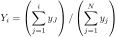
There are a number of test statistics based on the empirical distribution function (EDF). The EDF is the cumulative spectrum :
 |
(B.35) |
for the data and
 |
(B.36) |
for the model.
The EDF can be plotted using plot icounts. The best known of these tests is Kolmogorov-Smirnov whose statistic is simply the largest difference between the observed and model EDFs :
 |
(B.37) |
The XSPEC statistic test ks option returns  . The significance of
the ks value can be determined using the goodness command. In
general, the Kolmogorov-Smirnov test is not particularly powerful and
the next two test statistics are preferred.
. The significance of
the ks value can be determined using the goodness command. In
general, the Kolmogorov-Smirnov test is not particularly powerful and
the next two test statistics are preferred.
Cramer-von Mises (cvm)
The Cramer-von Mises statistic is the sum of the squared differences of the EDFs :
 |
(B.38) |
The XSPEC statistic test cvm option returns  and its
significance should be determined using the goodness command.
and its
significance should be determined using the goodness command.
Anderson-Darling (ad)
Anderson-Darling is a modification of Cramer-von Mises which places more weight on the tails of distribution :
 |
(B.39) |
The XSPEC statistic test ad option returns and its
significance should be determined using the goodness command.
CUSUM (cusum)
The CUSUM statistic (Page, E.S. (1954, Biometrika, 41, 100)) is the difference between the largest and smallest differences between the model and data EDFs.
 |
(B.40) |
Runs (runs)
The Runs (or Wald-Wolfowitz) test checks that residuals are randomly
distributed above and below zero and do not cluster. Suppose  is the
number of channels with +ve residuals,
is the
number of channels with +ve residuals,  the number of channels with
negative residuals, and
the number of channels with
negative residuals, and  the number of runs then the Runs statistic
is :
the number of runs then the Runs statistic
is :
![$\displaystyle Runs = (R-\mu)/\sqrt{[(\mu-1)(\mu-2)/(N-1)]}$](img817.svg) |
(B.41) |
where :
 |
(B.42) |
and
 |
(B.43) |
The hypothesis that the residuals are randomly distributed can be
rejected if abs(Runs) exceeds a critical value. For large sample runs (where
and both exceed 10) the critical value is drawn from the
Normal distribution. For instance, for a test at the 5% significance
level, the hypothesis can be rejected if abs(Runs) exceeds 1.96.