
Come analyze HEASARC, IRSA, and MAST data in the cloud! The Fornax Initiative is now welcoming all interested beta users.


Rank- SVD Response Matrix Compression
For instruments with large response matrices – microcalorimeters
(XRISM Resolve, Athena X-IFU), gratings (XMM RGS, Chandra HETG)
and densely-sampled CCDs – the convolution step
 can dominate the per-fit
elapsed-time cost. XSPEC exposes an optional rank- Singular
Value Decomposition (SVD) compression of the RMF that replaces the
exact sparse SpMV with two BLAS-3 matrix products at a
user-chosen rank. The compression is built once offline (by the
ftsvdcmprmf program in HEASOFT) and stored as a
.svdmat.fits side-car file alongside the original RMF.
At fit time, attaching the side-car activates the rank- path
in convolveMany / convolveTransposeMany; the
original RMF is otherwise untouched.
can dominate the per-fit
elapsed-time cost. XSPEC exposes an optional rank- Singular
Value Decomposition (SVD) compression of the RMF that replaces the
exact sparse SpMV with two BLAS-3 matrix products at a
user-chosen rank. The compression is built once offline (by the
ftsvdcmprmf program in HEASOFT) and stored as a
.svdmat.fits side-car file alongside the original RMF.
At fit time, attaching the side-car activates the rank- path
in convolveMany / convolveTransposeMany; the
original RMF is otherwise untouched.
Whether this compression actually buys speed depends sensitively on the instrument; this section describes how to find out, how to use the feature, and what its known limits are.
The factorisation
Given the response matrix  of size
 (photon
energy bins by detector channels), the SVD is
(photon
energy bins by detector channels), the SVD is

 and
and  orthogonal and
  diagonal with non-
negative entries
diagonal with non-
negative entries
 .
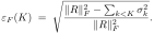
Truncating to the leading singular components gives the best
rank- approximation in the Frobenius norm:
.
Truncating to the leading singular components gives the best
rank- approximation in the Frobenius norm:

 is
is
 -element dot product plus a -element fan-out –
two BLAS-3 calls per fit step. When
-element dot product plus a -element fan-out –
two BLAS-3 calls per fit step. When
 and
the per-call flops are dominated by the second sum,
convolveMany is asymptotically
and
the per-call flops are dominated by the second sum,
convolveMany is asymptotically
 times faster than the exact path (
 = number of noticed
channels).
= number of noticed
channels).
Building a side-car
The HEASOFT task ftsvdcmprmf reads an OGIP RMF and writes a .svdmat.fits side-car:
ftsvdcmprmf  infile=  outfile=
            [arffile=]
            [eps=1e-4]   [kmax=256]
            [oversamp=10] [powiter=2]
            [check=yes]  [nprobes=8]
            [emitrmf=]   [emitthresh=1e-10]
The build uses Halko-Martinsson randomised SVD, which is
 in flops with a small (1–8) multiplicative oversample. Default
parameters target
in flops with a small (1–8) multiplicative oversample. Default
parameters target
 at
at
 ; the
build prints the actual rank retained and the achieved error.
The check step compares the rank- reconstruction
against the exact RMF on random probe vectors and reports the
worst-case relative error – a fast sanity check.
; the
build prints the actual rank retained and the achieved error.
The check step compares the rank- reconstruction
against the exact RMF on random probe vectors and reports the
worst-case relative error – a fast sanity check.
The emitrmf parameter is unrelated to the side-car path;
it writes a sparse OGIP RMF reconstructed from  with entries
below emitthresh dropped. This is the “denoising”
use-case (NuSTAR-style responses assembled from Monte-Carlo
simulations, where the tail components carry numerical noise) and
produces a drop-in replacement RMF that does not require
side-car support to load.
with entries
below emitthresh dropped. This is the “denoising”
use-case (NuSTAR-style responses assembled from Monte-Carlo
simulations, where the tail components carry numerical noise) and
produces a drop-in replacement RMF that does not require
side-car support to load.
Attaching a side-car
In an XSPEC session, give the side-car path to response:
data 1:1 mysrc.pi
response 1 mysrc.rmf
arf 1 mysrc.arf
response 1 mysrc.svdmat.fits      ; attach side-car
The file format (RMF vs side-car) is autodetected by HDU
inspection. Attaching does not modify the underlying RMF, so
arithmetic on the exact RMF (response none, gain
shifts, ARF reloads) all continue to operate on the exact path.
At fit or hmc time the rank- path is dispatched
in convolveMany / convolveTransposeMany for the
attached response.
To switch back to the exact path, re-load the original RMF:
response 1 mysrc.rmf ; SVD cleared, exact path activeThe reload installs a fresh response object, which destroys the previously-attached side-car as a side-effect.
The rank chosen at attach time defaults to the smallest value
for which
 xset responseSvdEps
(default
xset responseSvdEps
(default  ). Two per-response overrides are recognised:
response 1 svdrank 128       ; pin K_eff = 128
response 1 svdeps  1e-3      ; pin eps target, auto-pick K_eff
Either override can be reverted by passing
 . Neither survives
a re-load of the underlying RMF.
. Neither survives
a re-load of the underlying RMF.
Hard-cap fallback
If the chosen
 is larger than
 , the SVD apply cost exceeds the exact sparse
SpMV cost; in that regime the side-car is attached but
not used – XSPEC logs a one-line warning and the exact
path runs as if no side-car were attached. This protects users
who attach a side-car built with a permissive
, the SVD apply cost exceeds the exact sparse
SpMV cost; in that regime the side-car is attached but
not used – XSPEC logs a one-line warning and the exact
path runs as if no side-car were attached. This protects users
who attach a side-car built with a permissive
 target on a non-compressible RMF. Override
response 1 svdrank <K> explicitly to force the rank-
path even past the hard cap (useful for the basin-finder
workflow described below).
target on a non-compressible RMF. Override
response 1 svdrank <K> explicitly to force the rank-
path even past the hard cap (useful for the basin-finder
workflow described below).
Whether your instrument benefits
The singular spectrum of an OGIP RMF varies enormously by instrument class:
- CCDs with broad redistribution (Chandra ACIS-S,
ASCA SIS, XMM EPIC-pn). Compress well to
 –
– at
at
 . Per-call convolve speedup
 –
–
 ; total fit speedup is smaller because
convolve is typically not the per-iteration bottleneck.
; total fit speedup is smaller because
convolve is typically not the per-iteration bottleneck.
- Microcalorimeters (XRISM Resolve, Athena X-IFU).
The matrix is band-Toeplitz with a near-Gaussian kernel and a
slow polynomial singular-value decay. At
 ,
,
 – the SVD path is useful only as a
“rough” preconditioner (see below), not for production fits.
– the SVD path is useful only as a
“rough” preconditioner (see below), not for production fits.
- Gratings (XMM RGS, Chandra HETG). Similar to
microcalorimeters – highly localised dispersive response with
slow singular-value decay.
- CdZnTe / Si hybrid (NuSTAR FPM). Slow decay,
though the denoising use-case (emitrmf from
ftsvdcmprmf) is valuable for cleaning Monte-Carlo noise
out of the tail.
A standalone Python audit tool at
Xspec/src/tools/rmf_rank_audit.py computes the
singular spectrum and
 table for any RMF and is
the recommended scout before committing to a build cadence.
table for any RMF and is
the recommended scout before committing to a build cadence.
The rough-then-exact workflow
At a rank where the SVD is too noisy for a production fit (high
on a microcalorimeter, say), the SVD path can
still be useful as a fast basin-finder when the initial-parameter
guess is far from the minimum. The cheap rank- steps move the
solution into the basin of attraction; the exact path then
refines:
xset query no
response 1 mysrc.svdmat.fits   ; attach
response 1 svdrank 250         ; force past hard cap if needed
fit 5                           ; cheap basin descent
response 1 mysrc.rmf            ; clear SVD
fit                             ; full-precision refinement
The xset query no matters: without it, the
“Number of trials exceeded: continue fitting?” prompt fires
under non-interactive EOF and silently bypasses the iteration
cap. An empirical example on the XRISM Resolve bvapec benchmark
fixture is in xspec_tests/results/branch2_svd_validation.md;
on that fixture the 5-iteration SVD phase + full exact phase ran
in  s vs
s vs  s for exact-alone from the same bad
initial guess.
s for exact-alone from the same bad
initial guess.
The right cadence (rank, iteration cap, switch-over criterion) is fixture-dependent and we deliberately do not ship a macro – the infrastructure above is enough to express it. See “Cross-checking the SVD path” for how to verify it.
Cross-checking the SVD path
Issue xset SVD_CROSS yes at the XSPEC prompt to make
every SVD-accelerated convolveMany and
convolveTransposeMany call also evaluate the exact path
and compare element-wise. The tolerance is
 relative; agreement outside
that envelope triggers a one-line warning naming the spectrum and
the worst-case bin. This is the analogue of the
CONVOLVEMANY_CROSS and VJP_CROSS xset
keys; it is off in production because the cross-check pays the
cost of both paths every step.
relative; agreement outside
that envelope triggers a one-line warning naming the spectrum and
the worst-case bin. This is the analogue of the
CONVOLVEMANY_CROSS and VJP_CROSS xset
keys; it is off in production because the cross-check pays the
cost of both paths every step.
The side-car file format
The .svdmat.fits file is a small binary table with three HDUs:
- SVDMAT_U –
 rows; each row is a
vector of length
rows; each row is a
vector of length  holding the
  -th left singular
vector.
-th left singular
vector.
- SVDMAT_V –
rows; each row is a
vector of length
 holding the -th right singular
vector.
holding the -th right singular
vector.
- SVDMAT_SIGMA –
rows; columns
K, SIGMA, EPS_F_AT_K.
Plus a primary HDU with provenance keywords identifying the source RMF (and optional baked-in ARF), the build version, the randomised-SVD seed, and the OGIP TELESCOP / INSTRUMENT / DETECTOR / FILTER strings that the side-car will be sanity- checked against at attach time. The format is read and written by the heasp::svdrmf class; see HEASOFT's heacore/heasp/svdrmf.h for the C++ API and Xspec/src/help/convolve_optimisation_design.md revision 2 for the full design rationale.